Two modes of operation have been defined. The proportional mode (range to audio feature mapping), provides the user with a general knowledge regarding both the close-by and distant surroundings through the detection of objects, doorways, depth discontinuities, etc. The derivative mode (temporal derivative of range to audio feature mapping), is used to obtain the greater detail necessary for shape and pattern detection.
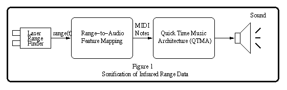
Figure 1 below illustrates the range data sonification process. The
user will scan their environment and obtain range measurements with the
laser range finder (LRF). Measurements are mapped to a particular feature
in the audio domain (see below). As most people are familiar with the notes
of the musical
scale [4], one feature we experimented with is frequency in the form
of MIDI (Musical Instrument Digital Interface) notes. Another feature experimented
with is amplitude (or velocity in terms of Midi). Finally, the MIDI note
is output using one of the 128 instruments available with the Quick Time
Music Architecture (QTMA) software synthesizer.
While in the proportional mode of operation, range measurements obtained with the LRF are mapped inversely to frequency using a logarithmic mapping. The frequency obtained from the mapping is then converted to its closest MIDI note value (see below for further details) and output for a specific duration.
With the derivative mode of operation, range measurements are not mapped to frequency directly but rather the change between consecutive range measurements is mapped inversely to frequency once again using a logarithmic mapping. As with the proportional mode, the frequency is converted to a MIDI note and output. In addition, with either mode of operation, the range measurement may optionally be mapped to the velocity (amplitude) of the Midi note in conduction with the frequency providing the user with an additional cue.
There were several different distance-to-frequency (or change in distance
to frequency) mappings
experimented with including linear and inverse square). In addition
to finding the output tones produced
with the logarithmic mapping pleasing, an informal lab survey of several
colleagues found they all
preferred the logarithmic mapping over the inverse square and linear
mapping. Table 1 below illustrates the various mappings currently
being used.
|
|
|
|||
|
|
|
|||
|
|
|
|
|
|
|
|
|
|
|
|
|
|
if d less than r:
F = kc-(d - r) a else F = F1 where: distance = d min.distance=r
|
if delta(d) less than
s:
F =kc-(D d - s)a else F = F1 where: max. distance=s |
|
|
Since there are no general guidelines for sonifying data [9], several different range-to-audio (or change in range to audio) mappings were experimented with. In the case of range to frequency, the output produced with a logarithmic mapping was most effective as it stressed range measurements close-by, but allowed for a perceived change in frequency throughout the entire range (non-logarithmic mappings are described in [5]). With the velocity (amplitude) mapping, a modified version of the inverse square law was used allowing for perceived change in velocity throughout the entire range of measurements. It was also decided to vary the frequency and velocity inversely with distance (allowing the frequency or velocity to increase as the distance or change in distance decreases), since the higher frequency/velocity notes can better 'grab' the attention of the user signaling of an object close-by).
The maximum frequency used in all of the mappings is 4000Hz corresponding to MIDI note 107 (which is actually 3951Hz). Frequencies above this level, using the present equipment, results in poor sound quality. Moreover, human perception of higher frequencies steadily deteriorates after age 30 and it has been estimated that 65% of visually impaired and partially sighted people are over 70 years of age [7]. The minimum frequency used was less restrictive and depended on which instrument was used to generate the sound output. For example, many of the bass instruments allow for a frequency as low as 32Hz (midi note value of 24).
Rather than map the range measurements directly to MIDI notes, it was decided to map the range measurements to frequency and convert the frequency to the closest corresponding Midi note in order to allow for greater flexibility with the actual mappings (e.g. easily modify the constant values used with the mappings to allow for various curves).
The sound output may be generated using Apple's sound manager or the
Quick Time Music Architecture. Although they are both similar (e.g.
both allow for the output of the 128 Midi notes), the sounds produced using
the QTMA far exceed the quality of sounds produced using the the Macintosh's
Sound Manager. In addition, the QTMA allows for the option of sound
generation using many different instruments and depending on the instrument
used the output can be very pleasant to listen to.
Velocity (Amplitude) Mapping
As mentioned above, the user may choose to alter the velocity (loudness) of the note being output inversely with range, providing an additional cue to object detection/recognition. Midi velocity values range from 0 (non audible) to 127 (too loud) however best results were achieved using a range of approximately 40 to 100 as velocity values below 40 are very weak and velocity values greater than 100 are too loud. As with the frequency mappings, several different range (or change in range) measurement mappings were experimented with including linear and logarithmic. For both modes of operation the best results were obtained using a modified version of the inverse square law.
Although the decrease of power followed by a wave follows the inverse square law, using the original inverse square formula, it was found that the velocity associated with the larger measurements were greatly reduced to the point where they are not audible. For example, (referring to the velocity mapping of table 1), when a = 100, the velocity corresponding to a range measurement of 10.00m is 1 causing the note to be non audible. To overcome this problem, the value of a can be increased, however, this will also increase the amplitude of the tones corresponding to the smaller distances to a point where they are too loud. Extremely loud tones may interfere with the (possibly important), environmental sounds the user hears (e.g. passing cars, people etc.). Substituting values less than two for 'b' allows for a uniform change in velocity throughout the entire range.
Regardless the number of range measurements taken per second, the time between consecutive readings is constant. As a result, each of the notes was output for the same duration (which was less than or equal to the duration between consecutive measurements). With both modes of operation, eight measurements per second were taken (a duration of 125ms). It was found however, that outputting each note for this same amount of time (thus producing a continuous note), resulted in a non pleasant output. Clicking noises were produced during the stopping of one note and beginning of the other and after several minutes the sound may become bothersome to the user. Outputting the tone for a duration of approximately 75% of the duration between measurements thus producing a small gap between consecutive notes, produced a more pleasant output.
Although the LRF allows for a maximum rate of 14 - 15 range measurements per second, as the rate is increased, the accuracy decreases. Even with the current setting of eight readings per second results in a noticeable loss of accuracy. For example, while obtaining measurements from a fixed position, and observing the LRF display, on can easily notice large fluctuations in consecutive measurements. This may pose a problem particularly while in the derivative mode as the purpose of this mode is to detect the finer detail not necessarily noticeable in the proportional mode. Reducing the rate of range measurements will increase the accuracy however, at a low enough rate, the sound output will not correspond to the current point of measure.
To overcome the above problems, Optic Systems will be donating a new Sentinel 3100 Laser Range Finder in the near future. This unit is capable of obtaining a maximum of 20 readings per second with an accuracy of 2 cm at this rate thereby allowing for the detection of finer detail and greatly reducing the possibility of the output not corresponding to the current point of measure.
Although the LRF's maximum range exceeds 100m, the maximum range for the purpose of this work was restricted to 15m with the proportional mode of operation. This restriction was placed to ensure the user is not overloaded with information and to restrict the range of notes output. For example an increase in the maximum allowable range measurement from 15m should also be followed by an increase in the range of frequencies used to ensure there is a perceived change in frequency throughout the entire range of allowable measurements.
At the other extreme, the minimum range measurement allowable was limited to 0.3m as it is used primarily for object detection/avoidance.
While in the proportional mode, range measurements are mapped inversely
to frequency using the logarithmic mapping shown in table 1 above.
Best results have been achieved when using the following constant values:
k = 4000Hz, c = 2.718 ('e'), a = 0.15 and r = 0.3m. Subtracting the
minimum distance from each distance reading ('r') to obtain the exponent
enables the frequency constant 'k' frequency to be used as the maximum
frequency. The exponent is then multiplied by a constant ('a'), to
increase the overall frequency for each reading. For example, without
this constant, a distance reading of 10.00m would result in a non audible
frequency of 0.25Hz, whereas using the constant a = 0.15 results in a frequency
of 933.6Hz. Both constants 'c' and 'a' were arbitrarily chosen.
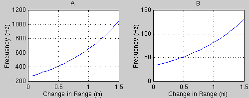
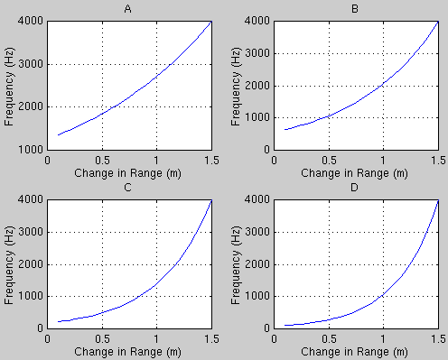
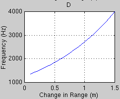
Various other values of 'c' and 'a' were experimented with and as
shown in figures 2 and 3 below, increasing the value of either 'c' or 'a'
causes a more drastic change in frequency for range measurements close
by and a smaller change in frequency for range measurements farther away.
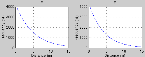
In addition to producing the most favourable results, the logarithmic mapping allowed for a perceived change in frequency throughout the entire distance range.
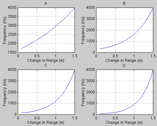
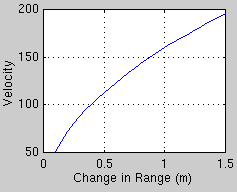
As with the frequency mapping, various arbitrarily chosen values were
substituted for the constants in the velocity mapping. As figure
4 below illustrates, decreasing the value of 'b' allows for a uniform change
in velocity throughout the entire range. Best results were achieved
using the following values: a = 75 and b = 0.4 (as shown in figure
4 diagram B).
Altering the velocity in conduction to the frequency provides an additional distance cue. In addition to a higher frequency note, the output note associated with distances close-by are also louder.
Depth discontinuity, or, a sudden change in depth, is defined as difference between the present and previous range measurement greater than a pre-defined value. It is important to convey such information to the user. For example, this could be used to locate a doorway with the door open since the distance to the object beyond the doorway (a wall etc.) will generally constitute a depth discontinuity.
Distance changes greater than 1.50m will result in a depth discontinuity.
It was found that using a value greater than this will prevent several
instances where there is a depth discontinuity from being conveyed to the
user. For example, by measuring the distance between several doorways and
the wall beyond, there were several instances where the depth discontinuity
is quite small (e.g. less than 2.0m), as shown in table 2 below:
|
|
|
|
|
|
|
|
|
|
|
|
|
|
|
To convey a depth discontinuity to the user, a signal unique from the regular output was used, ensuring it both "grabbed" the user's attention and was not mistaken as regular output.
Different notes to convey a Depth Discontinuity
High Timbre Note
Initially, the signal associated with a depth discontinuity was generated with the Square Wave data option of the Sound Manager. A low frequency (e.g. 100 Hz) and low amplitude (e.g. 60) note was output in the presence of a depth discontinuity. To ensure it was discriminable, the timbre of the note was raised to a maximum value of 255 allowing for a "buzzy" output.
Instrument From QTMA
Although the high timbre note was definitely discriminable, utilizing one of the instruments of the QTMA unique from the instrument used to generate the regular output (piano) to produce the output associated with a depth discontinuity produced far greater results. Various different instruments were experimented with including accordion, saxophone and oboe however, the drum cymbal at a frequency of 57Hz produced the greatest results. In addition to easily capturing the attention of the user once a depth discontinuity was detected it was also discriminable from the regular output produced with the piano. An informal lab survey of several colleagues found they preferred the output produced with the QTMA and were quickly and easily able to determine depth discontinuities. As a result, QTMA is used to generate the output associated with a depth discontinuity.
Reference Proportional Mapping
As mentioned in Appendix A - Optech Laser Range Finder, the accuracy
of the LRF is +/- 10cm. Since all range measurements are mapped to
the audio domain and output, ambiguities may arise and be particularly
noticeable when the LRF is focused on the same stationary location/object
for an amount of time. Although the range measurements should be
the same, due to the accuracy limitations, the measurements may fluctuate
as much as +/- 10cm. Such fluctuations would be noticeable to the
user. In an attempt to limit these fluctuations, this method defines space
known as the "No-Change Range" and every range measurement falling within
this space will not be mapped to the audio domain (e.g. there will not
be any output). When a range measurement does not fall within this
space, it is mapped as usual to frequency (and optionally velocity) and
the corresponding note is output as before. (Depth discontinuities
are treated as before).
Figure 5 below illustrates the algorithm to allow for such a
"space":
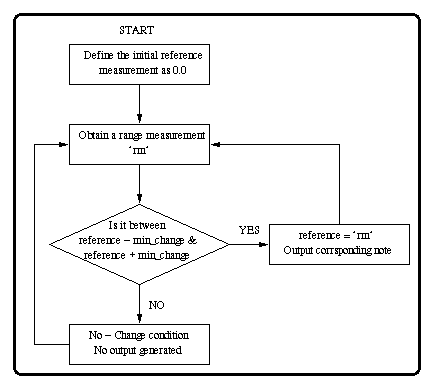
As shown in figure 5, initially we define the reference to be 0.0m.
As a result, the "space" is initially defined as 0.0m - min_change and
0.0m + min_change (where min_change represents the accuracy of the LRF
- 10cm). Upon obtaining the next change in range measurements ("change"),
a check is made to see whether this change is within the "space".
If it is, we define this as a "No-Change" condition and there is no sound
output generated. However, if it is not, then the range measurement
is mapped to the audio domain and the corresponding note is output (as
regularly done). In addition, we must now define a new "space".
The new space is defined by changing the value of the reference to "the
value of the current range measurement". Figure 6 below illustrates
the operation of this method.
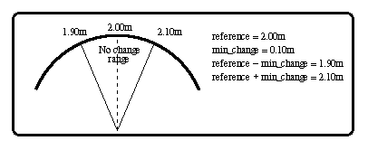
Consider the following:
reference = 2.00m
min_change = 0.10m (the accuracy of the
LRF)
current range measurement = 1.95m
reference - min_change = 2.00m - 0.10m = 1.9m
reference + min_change = 2.00m + 0.10m = 2.1m
Since current range measurement (1.95m), falls within the "space", there will not be any sound output. Now suppose the next range measurement is 6.10m. Since it does not fall within the range, it will be mapped to the audio domain using the mappings described previously and the corresponding note will be output. In addition, reference will be assigned the value of this measurement (e.g. reference = 6.10m).
While in the derivative mode, rather than using the range measurements themselves, the change between consecutive range measurements (an approximation to mapping the derivative of range as a function of time) are mapped to the audio domain. Although such information may not necessarily be used to locate objects, it could be used to provide a greater detail about the user's surroundings. For example, depth discontinuities will easily be detected, as there will be a sudden jump in the derivative between consecutive readings. At the other extreme, flat surfaces could also be detected as the derivative between consecutive range measurements will not change (or will change slightly).
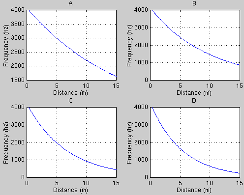
As another example, figure 7 below illustrates how this sonification could be used to detect corners. The change between consecutive range measurements (beginning at the point labeled 'Scanning Position'), of Wall X, will continue to increase until they reach a maximum value at the corner. Then while scanning Wall Y, (beginning from the corner), depending on the user's position relative to Wall X, the change between consecutive measurements will follow another pattern. In diagram A where the user's position is close to wall X, the change in consecutive range measurements will drop significantly within a small region, then level off and once again begin to increase. As shown in figure 7B, when farther away from Wall X, the change between range measurements will drop steadily while scanning Wall Y after encountering the corner. As a result, the sonification produced with such a mapping will result in a definite pattern (for example in figure 7B while scanning wall X towards the corner, the frequency of adjacent notes will increase until they reach a maximum at the corner and then decrease) which they user may interpret as the presence of a corner.
Irrespective of the user's scanning position, scanning at a faster rate
will result in a more drastic change between range measurements as opposed
to scanning at a slow speed.

Two forms of the derivative mapping were experimented with.
1) AbsoluteThe different versions of both absolute and non-absolute mappings experimented with are described in section below.
2) Non-Absolute
As mentioned above, there could be situations where the derivative remains constant (e.g. no change between consecutive measurements). This is defined as "No - Change" condition. Taking into account the accuracy of the LRF, the smallest change between consecutive measurements was restricted to 0.1m. Any difference less than 0.1m constitutes a "No -Change". For example consider two consecutive range readings of 2.41m and 2.49m. Since the change between the two measurements is less than 0.1m (e.g. 2.49m - 2.41m = 0.08m), this will result in a "No-Change" condition and may be conveyed to the user in one of two methods:
1) Generate Sound OutputGenerate Sound Output
2) Do Not Generate Any Sound Output
In the case of generating sound output for the "No-change" condition, it was decided to output a note generated with a unique instrument ensuring the user is aware of this condition. It has been observed that while scanning, many measurements result in a "No-Change" condition. To prevent the user from becoming overwhelmed (annoyed) by such output, the generated note was of a low frequency and low velocity. In addition to producing a more "pleasing" effect, it ensured the user is definitely aware of the note output when there was a change between consecutive range measurements (as this output is "stronger" and generated using a unique instrument).
Do not Generate Any Sound Output
In the case of "No sound generation", upon encountering a "No-Change" condition, there is simply no output generated at all. Although it definitely allows the user to become aware of a change (e.g. there will be a note output after a quiet period), this may also cause confusion as the user may mistake a long period of "No-Change" with a possible malfunction of the unit.
In addition to restricting the minimum allowable change between consecutive measurements (to 0.1m), it has been observed that the changes between consecutive measurements are generally small (less than 0.5m). As a result, the maximum change between consecutive measurements was restricted to an arbitrarily chosen 1.5m. For example, consider the following two range measurements of 3.55m and 6.55m. The difference between them is 6.55m - 3.55m = 3.00m however, the actual value mapped will be 1.5m. As shown in table 1, the maximum allowable change between consecutive range measurements is used in the (derivative mode) logarithmic frequency mapping. As a result, restricting the maximum allows for a more drastic change in frequency throughout the entire range allowing the user to discriminate between small changes. For example, consider the following three consecutive range measurements: 2.35m, 2.46m 2,58m. The first output will be generated based on the difference between 2.46m and 2.35m which is 0.11m. Although the next output (2.58m - 2.46m), based on a change of 0.12m is only 0.01m the note output in each case will be different allowing the user to discriminate such a small change.
With the absolute mapping, the absolute value of the change in range measurements was mapped to frequency and/or amplitude. As shown in table 1, the change in range measurements was mapped inversely to frequency using a logarithmic mapping and optionally to velocity (amplitude) using a modified version of the inverse square law mapping.
With this mapping, the change in consecutive range measurements was
simply mapped to frequency and optionally velocity. As with the proportional
mode of operation, a logarithmic mapping was used to map the change in
range measurements to frequency (see table 1). Various different
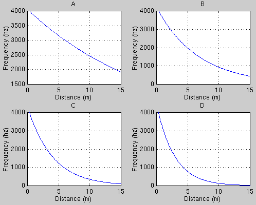
constant values were experimented with and once again as with the proportional
mode mapping, increasing the value of 'c' and 'a' caused an increase in
the overall range of frequencies and allows for a more "drastic" change
in frequency. The graphs of figures 8 and 9 below illustrate this
effect.
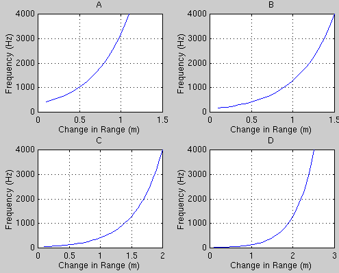
Likewise, as shown in figure 10 below, the same effect is achieved by
decreasing the value of 'r' (which represents the maximum allowable change
in range measurements). It has been observed smaller values of 'r'
(less than 2.0), allow for easier corner detection as there will be a definite
perceivable change in frequency between consecutive tones even with a small
change in distance.
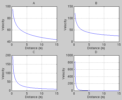
As with the proportional mode, the velocity of the note may optionally
be altered using a modified version of the inverse square law. As
shown in Figure 12 below, the following constant values allowed for a uniform
change throughout the entire range: a = 100 and b =0.4. This allowed
velocity to range from 33 (corresponding to the minimum change in range
measurement of 0.1) to 107 (corresponding to the maximum allowable change
in range measurements of 1.5).

The non-absolute mapping considered whether the change in range measurements
is positive or negative. A positive change indicates the location being
measured is farther away from the user relative to the last location (i.e.
the current measurement is greater than the previous measurement). A negative
change indicates that the location being measured is closer to the user
(i.e. the current measurement is less than the previous measurement). Such
information was conveyed with distinct signals ensuring the user could
easily discriminate among them.
Frequency
Piece-Wise Constant Non-Absolute Mapping
Frequency remained piece wise constant (e.g. a different constant frequency
for changes "coming closer" and "moving farther"), while the amplitude
was mapped inversely to the change in range measurements.
Various different constant frequency values were experimented with
however, best results were obtained when the difference between the frequencies
were large (e.g. 200Hz and 3000Hz), ensuring the user is able to discriminate
them. It was decided to use the low frequency (261.625Hz - Midi note
60 - Middle C), in the case of the change in measurements moving away (e.g.
the change is positive) and the higher frequency (3500Hz - Midi note 96),
for coming closer (e.g. the change in measurements is negative).
To map the amplitude, the modified inverse square law was used as shown
in table 1. Whether the change in range measurements was "moving
closer" or "moving farther", the amplitude increased as the change became
larger positive or negative (e.g. the amplitude associated with a change
of -1.5 was larger than an amplitude associated with -0.5). Various
exponent values were experimented and it was observed that increasing the
value of the exponent resulted in a drastic amplitude change for a small
portion of the range (e.g. for large changes in range measurement) while
the amplitude changed slightly for small changes in range measurement).
Figure 13 below illustrates the the change in range vs. velocity curve
produced using the values of a = 160, b= 0.5.
In the case of a "No-change" condition, both sound output and no sound output was used. In the case of sound output, it was decided to use a frequency in between the other two frequencies (e.g. 1600Hz). In addition to being discriminable, it may also be used a reference note as when a change is encountered, the frequency will be either higher or lower than the No-change note.
This method was implemented using the Apple Sound Manager as it allows for a much greater range of amplitude values (0 - 255) as opposed to Quick Time which is limited from 0 to 127. The small velocity range available with Quick Time made it difficult to perceive the magnitude of the change in measurements (e.g. a change of 0.2 was almost as loud as a change of 0.25). Using the Sound manager however, produced pleasant effects.
Different Instrument Non-Absolute Mapping
Rather than using "piece-wise" constant frequencies as described above, in this method, the frequency in addition to the velocity (amplitude) of the note was mapped to the change in range measurement. A distinct instrument was used to convey the changes in range measurements "moving closer" while another was used to convey changes "moving farther". In both cases, the frequency (and optionally velocity) was altered inversely to the change in range measurements using the same mappings used as the regular absolute mapping described above. As with the regular absolute mapping, best results were achieved using the following constant values:
Using different instruments to convey the derivative information was a definite improvement over the previous piece-wise constant frequency method described above. Depending on the two instruments used, there will not be any confusion as to whether the change in range is either "moving closer" or "moving farther". However, when the instruments are similar (e.g. church organ and electric organ, or guitar and electric guitar) it is difficult to discriminate amongst the two conditions as the output is very similar. Various instrument combinations were experimented with. Best results were achieved using the "Fretless Bass" to generate the output associated with changes "moving farther" and a "Koto" to generate the output associated with changes "coming closer".
Different Instrument with Different Frequency Ranges Non-Absolute Mapping
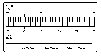
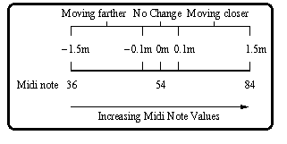
This mapping takes advantage of most peoples familiarity with the notes of the musical scale [4]. A region of notes from the musical scale was associated with changes moving closer and a different region of notes for changes moving farther away. Each range consisted of two octaves (24 notes) and was separated by a single octave. As shown in figure 16, the range associated for positive changes in range (e.g. moving farther) begins with MIDI note 24 (32.7Hz) and ends with Midi note 48 (130.8Hz). The range associated with a negative change in range measurements (e.g. moving closer) begins with Midi note 60 (261.625Hz) and ends with Midi note 84 (1046.5Hz). The octave in between (midi note 49 - 60) separates the two regions ensuring there is no confusion as to which region an output tone belongs to. As with the previous mapping described, different instruments were used to generate the output depending on whether the change in range was positive (moving farther) or negative (moving closer).
As with the previous mappings, in the case of a "No-change" condition, both output and no-output were experimented with. In the case of generating output for the "No-change" condition, best results were achieved when using Midi note 54 (185Hz). This note falls in the middle of the combined ranges and actas as a reference note allowing the the user to better discriminate amongst the notes in each of the regions (e.g. any note output with a lower frequency than Midi note 54 must be from the lower region associated with changes moving away). The velocity of this No-change note was kept low (50) ensuring the output did not become bothersome to the user.
Rather than mapping the changes in range to frequency and then convert the frequency to the closest Midi note, a linear mapping was used in which the change in range was mapped directly (e.g. not inversely) to the Midi notes in the corresponding region. The following formula was used to map the change in range to Midi note:
In the case of "moving closer", the following values were substituted in the above formula:Midi note = (r / (range / N)) + awhere:
r = change in range between current and previous measurements
range = maximum allowable change - minimum allowable change
N = number of keys the region contains
a = minimum Midi note of the particular range
In the case of "moving farther" the following values were used:range = 1.5m - 0.1m = 0.14m
a = 24
N = 24Midi note = (r / (0.14m / 24)) + 24)
Using the above formula allows the range of notes as well as the min/max allowable change in range to be easily increased/decreased. Only the corresponding variables must be altered to reflect any change - the formula will work correctly.range = 1.5m - 0.14m = 1.4m
a = 60
N = 24Midi note = (r / (0.14m / 60)) + 24)
Using the above mapping in the case of "moving closer" larger changes
in range corresponded to a larger Midi note as expected. However,
in the case of "moving closer", larger changes in range correspond to smaller
Midi notes while smaller changes correspond to larger Midi notes.
This may be easily changed by modifying the formula used in the case of
"moving farther" however it was decided against altering it since as shown
in figure 14 below, we now have a continuous range from -1.5m to 1.5m where
the frequency increases as the change between measurements increase.
It takes a little practice to become acquainted with the idea of larger
changes in range moving away correspond to smaller frequencies. This
may be due to the fact that with all previous mappings larger changes in
range corresponded to higher frequencies. Regardless, after several
minutes of use, we familiarized ourselves with the mapping and actually
enjoyed it. In the case of corner detection, referring to figure
7, while scanning Wall X moving towards the corner, the changes in range
measurements will be increasing. Since they are "moving away", the
Midi notes will be decreasing (e.g. decreasing frequency) until they reach
a minimum at the corner. While scanning Wall Y beginning from the
corner, it is usually the case that the first range measurement encountered
on Wall Y is less than the measurement obtained at the corner which will
result in a negative difference (e.g. moving closer). As a result,
this note will be at a much higher frequency than the note corresponding
to the corner measurement and it will also be generated using a different
instrument. Both these factors allow for corners to be detected easier
than before.