SUMMER AUDIO RESEARCH REPORT 1997
by Bill Kapralos
(under the supervision of Professor E.
Milios)
Table Of Contents:
1 Introduction
2 Equipment
2.1
Workstation
2.2 Headphones and Speakers
2.3
Optech Laser Range Finder (LRF)
2.3.1 Operation of the LRF
2.3.1.1 Power
2.3.1.2
Turning the Unit on (Obtaining a Reading)
2.3.1.3 LRF Messages
2.3.1.4 Remote
Terminal Connection
2.3.1.5
Control Commands Via a Serial Connection
2.3.1.6
Description of the Serial Port Data Transmitted
2.3.1.7 LRF Specifications
3 Source Code
3.1
lrf_functions.h
3.2
lrf_functions.c
3.2.1
intSerialPortInit(char *serialPortName)
3.2.2.
int sendCommand(char *cmnd, int cmdLength)
3.2.3. int
fdHasCharacters(int fileDes)
3.2.4.
int getReading(unsigned char *buffer)
3.2.5.
float processReading(unsigned char* reading)
3.2.6 void lrfSetUp()
3.2.7
double calcAvgDistance(double *readings, int numOfReadings)
3.2.8
void error(char * errorMsg)
3.3
lrf_audiov2.h
3.4.
lrf_audiov2.c
3.4.1.
int audioInit(char *audioDevice, char *audioCntrlDevice)
3.4.2
int sendAudio(short *buffer, int numOfSamples)
3.4.3
void tableInit(short *table[], int varyMagnitude)
3.4.4
short *makeWave(double frequency, double magnitude)
3.4.5
short *makeDepthSignal(in numOfSamples)
3.4.6
short *createNoise(int numOfSamples, double excitation)
3.5
lrf_main.c (Executable name: lrf)
3.6
lrfCont.c (Executable name: lrfCont)
3.7
lrf_piano.c (Executable name: lrfPiano)
3.8
Makefiles
3.9
Additional Code Written
3.9.1
playTone.c (Executable name: tone frequency [magnitude])
3.9.2 cosLookUp.c
3.9.3 Time Taken to Execute
Portions of Code
3.10
Program Requirements
4
Sound Output
4.1 Sample Rate
4.2
Audio Encoding and Sample Precision
4.3
Distance to Frequency Mappings
4.3.1 Linear Mapping
4.3.2 Inverse
Square Mapping
4.3.3 Logarithmic
Mapping
4.3.4 Piano Keyboard Frequencies
4.4
Distance to Mangnitude Mapping
4.4.1 Inverse
Square Law Mapping
4.5 Generation of the Samples
4.5.1 Output of a Continuous Tone
4.6
Real-Time Sample Generation vs. Wave look-up Table
4.7
Depth Discontinuity
4.7.1 Summation
of Sine Waves
4.7.2 Triangular
and Pulse Signals
4.7.2.1
Probability: The Triangular Distribution
4.7.2.2 Triangular
Formula
4.7.3
Using and Average of the 'N' Previous Distances
5
Internet Sites Visited
5.1
Related Research (past and present)
5.1.1 Obstacle Detectors
5.1.2
Orientation and navigational Aids
5.1.3 Environmental
Aids
5.1.4 Virtual Sound
5.2 Commercial Products
5.3 MIDI Sites
5.4 Miscellaneous
Sites
5.4.1 Linksa
to Related Sites
5.5 Newsgroups
6
Suggestions and Conclusions
6.1
Ideas for Future Continuation of the Project
6.1.1
Use of MIDI to Generate Sound
6.1.2
Use of a Macintosh over the SUN Workstation
6.1.3
Eliminating the Effects of the "Curves of Equal loudness"
6.1.4 New 'Power' and
'Data Out' Connectors
6.2 Conclusions
6.3 Acknowledgements
7 References
7.1 Bibliography
7.2 Source Code
Refernces
1. INTRODUCTION:
The visually impaired rely on non-visual senses, primarily hearing,
to help them locate and identify objects within their immediate and distant
environment Although all of the senses are able to convey information
pertaining to an object (i.e. texture, temperature, size), only the auditory
system is capable of providing significant distance cues (coded primarily
through intensity). Most objects do not emit sounds, however, they
are capable of reflecting sound coming from other sound sources allowing
the intensity of these reflecting sounds (echoes) to be used as distance
cues. Although these echoes may provide information about an object's
distance, sound emitting sources may not always be present.
In an attempt to imitate these natural occurring distance cues,
several devices have been developed in which the distance of a person to
an object is conveyed to the user through sound. Most of these devices
make use of sonar in which an ultrasonic sound is emitted from the device
and the time taken for the echo to return is directly related to the distance
of the reflecting object.
In the spring of '97 Professor Milios proposed that I investigate
the conversion of distance of an object into audible sound as a summer
research project.
Distance measurements could be easily obtained using the Optech
Laser Range Finder (a high accuracy infrared ranging device).
Therefore goal of my project was to obtain these distance readings and
convert them into audible sound ultimately leading to a product which will
aid the visually impaired with their travel and mobility.
The following pages describe the work I have completed during this four
month summer period.
2. EQUIPMENT:
2.1 WORKSTATION
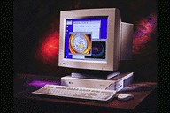
Either the SUN Ultra 1 or the SUN SparcStation 5 workstation was used.
The software written for this project is compatible with both. Each
workstation contains two serial ports (A and B) and each serial port contains
a 25 pin female RS-232-C compatible connector. The serial ports can
be accessed with the following names:
-
Port A: "dev/ttya"
-
Port B: "dev/ttyb"
The workstations contain one audio port each and can be accessed with the
name "dev/audio".
2.2 HEADPHONES AND SPEAKER
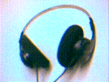
The sound may be output with the workstation's built-in-speaker or with
headphones. Panasonic XBS headphones were used and allowed for a
greater quality of sound compared to the built-in-speaker especially with
the frequencies above 4kHz.
2.3 OPTECH LASER RANGE
FINDER (LRF)
Optech Laser Range Finger (LRF) model G-150 is used to obtain the distance
readings. "The Rangefinder contains an infrared laser source emitting
infrared radiation invisible to the human eye (890 nanometeres) and should
not be viewed directly with the eye or with optical devices when the laser
is firing ." (Model G-150 owner's manual).
2.3.1 OPERATION
2.3.1.1 POWER
The LRF is powered by an external 12V battery source. A fully charged
battery will provide approximately 16 hours of operation and requires 18-24
hours to become fully re-charged. The LRF warns the user of a low battery
by using a '*' instead of the decimal point when giving a reading.
For example, a distance of 2.43 will be given as 2*43. I have found
that about 2 hours of battery life remain upon receiving the initial '*'.
After this warning period, the LRF will no longer obtain readings and will
issue an error message (ERROR 1b). On several occasions, the 'battery
low' warning failed to appear prior to the error code.
2.3.1.2
TURNING THE UNIT ON (OBTAINING A READING)
Upon turning the unit ON, the LASER ON LED (see figure 2.1 below) will
light and a brief self-test routine will be conducted. If the self
test reveals a problem with the unit then an error message appears on
the display. The only error code encountered was 'ERROR 1b' which
indicates that the battery requires charging. If the self-test is
passed, the LASER ON LED goes off and 'READY' appears on the display until
measurements begin. Measurements can be initiated in one of two ways:
1. Manually:
By pressing the START button to obtain a single measurement (Single
update mode) or can be set to take continuous readings (Continuous update
mode) by installing the DATA IN adapter plug. Plugging in the adapter
plug prior to turning the unit ON results in readings being
taken immediately following power ON without pressing
the START button.
2. Computer:
A computer generated "start" pulse signal (any positive going pulse)
can be sent to the LRF by a remote computer to initiate a reading (Single
update mode). Continuous update mode can also be achieved by sending
the appropriate command (see table 2.2 for a list of the available commands).
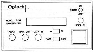 Figure 2.1
Model G-150 Laser Range Finder Control Panel.
Reprinted from the G-150 owner's manual.
Figure 2.1
Model G-150 Laser Range Finder Control Panel.
Reprinted from the G-150 owner's manual.
2.3.1.3 LRF MESSAGES
1. DISPLAY MESSAGES:
READY
Indicates the unit has passed its self-test and can begin taking reading.
*
Replaces the decimal point in a range reading to indicate the battery
is low
(below9.5V). Appears on the display as well as the remote
terminal.
<
Appears to the left of the range reading indicating the over 12.5% of the
shots were
invalid (drop-outs). This is ignored in my present program
implementation.
<<<<
Appears in place of a reading (both on the display and the remote terminal)
indicating an accurate reading could not be taken.
ERROR
Appears on the display when there is a problem with the unit..
2. BEEPER
-
1 SHORT BEEP Normal reading
obtained.
-
2 SHORT BEEPS Valid reading however,
more than 12.5% shots were drop outs. .
A '<' also appears on the display.
-
1 LONG BEEP
Unable to take an accurate reading. '<<<<' also appears.
2.3.1.4 REMOTE TERMINAL
CONNECTION
The LRF is capable of asynchronous serial data communications through the
connection of the DATA OUT cable (containing a D9S female connector) to
a remote computer. The Sun workstation contains a 25 pin female connector,
therefore, to connect the workstation to the LRF, a 25 pin male to 9 pin
male connector is required.
Several of the solder connections on the D9S became loose and were re-soldered.
To avoid any wiring mix-up, table 2.1 below shows the correspondence between
colour wire coming from the six pin circular connection and the pin number
of the D9S connector
|
PIN NUMBER
|
WIRE COLOR
|
|
2
|
Green
|
|
3
|
Brown
|
|
5
|
Black
|
|
9
|
Red
|
Table 2.1
DATA OUT to D9S Connector
Both the POWER and the DATA OUT connectors are 'snap-lock circular
connectors'. I experienced difficulties with both connectors.
For example, readings failed to be transferred to the computer even though
they appeared on the LRF display and occasionally the power turns ON/OFF.
By taping the wiring of both connectors to the LRF, I was able to temporarily
correct these problems. I suspect the problems are due to loose wire
connections on the circular connector, however I was unable to open the
connectors to verify and correct the problems.
2.3.1.5
CONTROL COMMANDS VIA A SERIAL CONNECTION
Upon turning the unit ON, the LRF is in its default mode (controlled by
its front panel switches) even if a serial connection with a remote terminal
exists. To override the default mode the LRF must receive a control
command. There are six control commands available in addition to
the programmable shots/reading command (see table 2.2).
The commands can be sent at any time and in any order however, all the
commands must contain a Carriage Return (CR) as their last character.
In order to process each command, the LRF requires a certain time delay.
According to the Optech manual, this delay should be 200usec, however,
I discovered the delay time required is about 1ms.
This does not affect the proper functioning of my program since commands
are issued once only prior to obtaining any readings.
|
DESCRIPTION
|
COMMAND LINE
|
|
BEEPER ON
|
'B'
|
|
BEEPER OFF
|
'Q'
|
|
SINGLE UPDATE
|
'S'
|
|
CONT. UPDATE
|
'C'
|
|
OUTPUT IN METRES
|
'M'
|
|
OUTPUT IN FEET
|
'F'
|
Table 2.2
LRF Command Codes
Each command must be followed by a Carriage Return
("\r"). A computer may send
both the command and the Carriage Return together
enclosed in quotes. (e.g. "B\r").
2.3.1.6
DESCRIPTION OF THE SERIAL PORT DATA TRANSMITTED
All readings (including 'drop-outs') consist of nine ASCII characters.
The first is an SP and the last two are CR and LF (SP, CR and LF are ASCII
characters representing a space, line feed and carriage return respectively).
Depending on whether a reading is valid or a drop-out, the remaining characters
in between are as follows:
VALID READING:
Three characters representing the whole portion of the reading, a character
representing an ASCII period
followed by two characters representing the decimal portion.
When the whole portion of the reading requires less than three digits,
the character(s) not used are assigned SP.
DROP-OUT READING:
four ASCII characters representing '(', followed by two SP characters.
NOTE: With a terminal connection to the LRF,
upon turning the LRF ON, the ASCII characters
representing the string 'READY' are sent to the terminal.
2.3.1.7 LRF SPECIFICATIONS
1. RANGE
-
Distance readings can range from 0.2m to 100m. For my purposes, a
range between 0.5m and 15m was used. I have also found trying to
obtain a distance reading less than 0.2m results in a drop-out (indicated
by '<<<<').
2. ACCURACY
-
An accuracy of ?10cm is achieved between the temperature ranges of -20oC
and 50oC.
3. MEASUREMENT TIME
-
The FAST/SLOW switch sets the time taken to obtain a reading by controlling
the number of shots being averaged (each distance reading is an average
of all the shots fired in order to reduce random errors).
-
Two readings/second are obtained in the SLOW setting (1000 shots/reading),
while eight readings/second in the FAST setting (150 shots/reading).
With a serial connection many more shots/reading settings are permitted.
-
With a serial connection, during power ON the unit will respond to the
SLOW/FAST setting, however, this can be changed by sending the desired
shots/reading at any time. Valid settings can range from 1-9999
and must be followed by a Carriage Return ("\r"). For example, for
a setting of 150 shots/reading, "150\r" should be sent.
-
Decreasing the number of shots/reading decreases the time to obtain
a reading, however, it also reduces the accuracy of the distance readings.
4. ENVIRONMENTAL CONDITIONS
-
The LRF was used primarily during the day although I have experimented
with it during the night with a minimum amount of available light and have
found it works fine.
-
I have not had the chance to use the LRF during a snowfall or rainfall
although according to the owner?s manual, it should work fine.
-
Windows pose a problem with object recognition since the LRF will not measure
the distance to a window. Windows do not reflect the signal instead the
signal passes through the window and a measurement of an object beyond
the window is taken.
Further information regarding the Laser Range Finder can be found in the
following available documents:
-
"Model G150 Rangefinder User Manual" Version 1.1, May 1991
-
"Model G150 Release Notes" June 11 1992
For parts/service regarding the LRF, contact the following person:
Bob Karwal
Optech Systems
701 Petrolia Road
North York, Ontario
M3J 2N6
Tel: (416)661 - 5904
Fax: (416)661 - 4168
3. SOURCE CODE
Contains function prototypes and constant definitions used in lrf_functions.c.
Various functions (see below), to allow communication with the range finder
and to allow the processing of any data obtained from the LRF.
3.2.1 intSerialPortInit(char
*serialPortName)
Open and initialise the serial port using the following settings:
(Since there are multiple serial ports available on the workstations, the
device name is supplied by the caller of the function).
-
DATA SPEED:
9600 Baud
-
NUMBER OF DATA BYTES:
8
-
NUMBER OF STOP BITS:
1
-
PARITY:
NONE
-
MIN NUMBER OF BYTES TO APPEAR: 0
-
TIME TO WAIT FOR DATA:
0
All the above settings are contained in the 'termios' structure (as defined
in <termios.h>). The setting 'TIME TO WAIT FOR DATA' refers to
the minimum amount of time the 'read' call will wait for data to appear
at the serial port. The setting value supplied will be multiplied
by 10ms to determine the total wait time. The setting 'MIN NUMBER
OF BYTES TO APPEAR' refers to the minimum number of bytes the 'read' command
must obtain before returning.
Both of the above parameters are set to 0 since readings from the LRF
are obtained only when data appears at the port (see function fdHasCharacters()
below). .
Upon successful opening/initialisation, a 1 is returned otherwise 0
is returned signifying an error.
Further documentation regarding the serial port can be found in the
manual pages under the following titles:
-
termios
-
ioctl
-
fcntl
-
open(2)
3.2.2 int
sendCommand(char *cmnd, int cmdLength)
Send data (representing a command), to the LRF and delay the required time
allowing the command to be processed. The LRF will ignore any commands
it does not understand.
3.2.3 int fdHasCharacters(int
fileDes)
Returns the number of bytes available to be read from the serial port or
-1 if an error is encountered.
3.2.4 int getReading(unsigned
char *buffer)
Obtains a reading from the LRF (if available). Prior to reading the
port, it is determined how many bytes are available (using fdHasCharacters()).
A maximum of one reading (10 bytes) can be obtained per call. Upon
obtaining a reading, a 1 is returned otherwise 0 is returned.
3.2.5
float processReading(unsigned char* reading)
Converts the string of ASCII digits obtained from the LRF to a floating
point value using the following algorithm:
-
Determine whether the reading is 'out-of-range'. Out-of-range readings
cannot be processed and result in a return of 0.0.
-
Process the digits to the left of the decimal point (whole number portion).
Any reading without a decimal point signifies an error and results in a
return of 0.0.
-
Process the digits to the right of the decimal point (fraction portion).
-
When the converted reading value is within the acceptable range, it is
returned otherwise either MIN_DISTANCE (when the reading is below MIN_DISTANCE
) or MAX_DISTANCE (when the reading is greater than the MAX_DISTANCE)
is returned.
3.2.6 void lrfSetUp()
Send any required operation commands to the LRF. The order the commands
are sent in this function should not be altered. Certain commands
require other commands to be in operation. For example, before setting
the number of 'shots per reading' (LRF_TIMEOUT command), and turning the
beep off (BEEPOFF command), the LRF must already be taking readings.
The LRF_TIMEOUT command can be sent any time after the LRF has been
triggered to take readings.
3.2.7
double calcAvgDistance(double *readings, int numOfReadings)
Returns an average of all values contained in 'readings'. 0.0 is
returned when 'readings' does not contain any values. This function
was used when experimenting using an average of the previous N distance
readings to compare with the current reading to determine whether a depth
discontinuity was encountered. (As explained in section 4.5.3, comparing
the present distance with an average of the previous N distances may result
in a valid depth discontinuity not being conveyed).
3.2.8 void error(char *
errorMsg)
Display the message 'errorMsg' to the standard error (stderr), close the
audio and serial ports and exit the program. This function is called
when an error is encountered by the caller.
Contains function prototypes and constant definitions used in lrf_audiov2.c.
This file contains functions related to the audio port. Routines
to open, close, write to, and control the audio port as well as routines
to generate several types of audio signals are included.
3.4.1 Int audioInit(char *audioDevice, char *audioCntrlDevice)
Open and initialise the audio port with the following settings (all settings
are kept in the audio_info structure 'audioInfo' defined in audioio.h).
Where the location of any constant definitions is not given, see audioio.h):
audioInfo.play.port = AUDIO_HEADPHONE
-
Controls the output of the audio port. Output can be sent to either
of the following:
-
. Workstation built in speaker (AUDIO_SPEAKER).
-
Headphone jack (AUDIO_HEADPHONE), to allow the use of headphones.
-
audioInfo.play.balance = AUDIO_MID_BALANCE
-
Control the volume between the left and right channels.
-
Values between 0 and 64 are accepted.
-
When set between AUDIO_LEFT_BALANCE (0) and AUDIO_MID_BALANCE (32),
the right channel will be reduced in proportion to the balance value.
-
When set between AUDIO_MID_BALANCE and AUDIO_RIGHT_BALANCE (64),
the left channel is reduced in proportion to the balance value.
-
audioInfo.play.gain = AUDIO_GAIN
-
Output volume control.
-
Values between 0 (AUDIO_MIN_GAIN) and 255 AUDIO_MAX_GAIN are accepted.
-
see lrf_functions.h for the definition of AUDIO_GAIN.
-
audioInfo.play.sample_rate = FREQ_SAMPLING_RATE;
-
Sampling frequency of the audio data (in samples per second).
-
Currently set to 22050Hz.
-
See lrf_functions.h for the definition of FREQ_SAMPLING_RATE.
-
See 'audiocs' in the manual pages for the allowable sample rates.
-
audioInfo.play.encoding = AUDIO_ENCODING_LINEAR;
-
Audio data representation can be set to the following:
-
1. Linear PCM (AUDIO_ENCODING_LINEAR).
2. u-Law (AUDIO_ENCODING_ULAW).
3. A-Law (AUDIO_ENCODING_ALAW).
-
Currently use Linear PCM 16-bit encoding (see section 4).
-
audioInfo.play.precision = SAMPLE_PRECISION;
-
Number of bits used to represent each audio sample.
-
Allowable sample values are 8, 16 or 32.
-
Currently set to 16 bits allowing for sample values between -32768 and
32767.
-
See lrf_functions.h for the definition of SAMPLE_PRECISION.
Only one process may open the audio port at a time (not a problem in my
implementation), however two processes may access the audio device simultaneously
if one opens it read-only and the other opens it write-only. The
device is opened for write-only in the present implementation as there
is no reading (recording), applications in this program.
A 1 will be returned upon successful opening and setting of the audio
port and 0 if any errors are encountered.
I have made limited use of the audio device. Many more settings
and uses are possible. For further information regarding the audio
device, see the manual pages under the following:
3.4.2
int sendAudio(short *buffer, int numOfSamples)
Sends 'numOfSamples' bytes to the audio port beginning at address
'buffer'. Audio port must be initialized and the number of bytes
actually written to the port must be the same as the number sent to
avoid an error.
Data sent to the audio port is not output immediately but rather kept
in a buffer and output only when the buffer is full. In order to
output the data sent to the audio port immediately, the buffer is flushed.
3.4.3
voidTableInit(short *table[], int varyMagnitude)
The samples required for each cosine wave are calculated and stored in
a table (allowing for future look up and use), prior to sending the START
command to initiate readings by the LRF. The table contains
samples of cosine waves corresponding to distances between MIN_DISTANCE
and MAX_DISTANCE (incremented by 0.10 since this is also the accuracy of
the LRF in the temperature range of -20 to 50 degrees Celsius).
3.4.4
short *makeWave(double frequency, double magnitude)
Create and return a buffer of samples representing a cosine wave of the
specified frequency and magnitude.
3.4.5 short
*makeDepthSignal(in numOfSamples)
Create and return a buffer of samples representing a short pulse in the
corresponding PCM values.
3.4.6
short * createNoise(int numOfSamples, double excitation)
Create and return a buffer of samples representing noise of a magnitude
given by 'excitation'. Noise is created by generating random integer
values (in the range of -32768 to 32767), for each of the samples.
3.5 lrf_main.c
(Executable name: lrf)
Establishes serial communications with the Laser Range Finder (LRF).
Continuously obtains readings from the LRF, looks up and sends the appropriate
samples representing a cosine wave to the audio port.
The samples for each cosine wave are stored in a table. When
a reading is obtained, it is mapped to the corresponding samples in the
table and output. There is a slight delay (~8 sec.) between the time of
program execution and the time the first reading is obtained, to allow
for the initialisation of the table.
A reading containing more than 12.5% 'drop-outs' (as indicated by a
')'), is treated as a valid reading. When an "out-of-range
reading is encountered (as indicated by '))))'), the tone corresponding
to the last valid reading is output.
The presence of a Depth Discontinuity (a change in distance greater
than a pre-defined amount between the current and last valid reading),
causes the output of a non-tone signal (pulse).
Prior to program execution, the LRF must be turned ON and in the "READY"
mode. Should the LRF be turned OFF, the program must be stopped and
re-executed. "CNTRL-C" to stop program execution.
3.6 lrfCont.c (Executable
name: lrfCont)
Same as lrf_main1.c (see above), however a continuous tone is output in
this version. When there are no readings available from the LRF the
tone corresponding to the last valid reading is output.
3.7 lrf_piano.c
(Executable name: lrfPiano)
Distance readings are mapped linearly to the frequencies of a piano keyboard
stored in a table. Upon obtaining the frequency, the samples are
created in real-time (they are not looked up in a cosine wave table), and
output.
3.8 Makefiles
Each of the three versions contains its own makefile (as shown below):
-
Version 1: makefile
-
Version2: makefileContinuous
-
Version3: makefilePiano
In addition to the 'main' program file, the following files are also required
for each of three makefiles
-
lrf_functions.o
-
lrf_audiov2.o
-
libaudio.a
and the functions lrf_functions.h and lrf_audiov2.h require the following
header files as well:
<unistd.h>
<ctype.h>
<errno.h>
<sys/termios.h>
<fcntl.h>
<time.h>
<sys/filio.h>
<stropts.h>
<stdio.h>
<sys/audioio.h> <sys/file.h>
<sys/ioctl.h>
<termios.h> <math.h>
<stdlib.h>
"audio_device.h" "audio_hdr.h"
3.9 ADDITIONAL CODE WRITTEN
3.9.1
playTone.c (Executable name: tone frequency [magnitude])
This program outputs a tone corresponding to a specific frequency and magnitude
as entered by the user through command line arguments. A value for
the magnitude is optional and if not entered, the tone is not scaled (e.g.
magnitude = 1).
This program was used to allow easy output of tones and could also
be used during experimentation to introduce subjects to the output they
will encounter..
The makefile for this program is makefileTone.
3.9.2 cosLookUp.c
Code to initialise and use the cosine-look-up table described in section
4.4. As mentioned, using the table increases the amount of time required
to determine the cosine of a specified radian value however, perhaps it
could be improved for future use.
3.9.3 TIME TAKEN
TO EXECUTE PORTIONS OF CODE
To ensure all readings taken by the LRF are actually processed before the
arrival of the next reading, the time required to process the reading
(look-up and output samples etc.), must be determined. Since the
function "getReading()", obtains only one reading at a time, a build up
of readings results when readings arrive faster than they can be processed.
This build up of readings will be processed on a "first come first serve"
basis and may result in the incorrect tone output for a particular distance.
The UNIX function 'gettimeofday()' returns the current time expressed
in elapsed seconds and microseconds since 00:00 Universal
Co-ordinated Time, January 1, 1970 (manual pages - gettimeofday).
To determine the time required to execute a segment of code, the time of
day is obtained just before the code segment is entered and subtracted
from the time of day obtained just after the execution of the code segment
as shown below:
#include <time.h>
struct timeval t1, t2;
int *temp = NULL;
gettimeofday (&t1, temp);
** CODE TO BE TIMED IS INSERTED HERE **
gettimeofday (&t2, temp);
printf ("Execution time: %5.3f s\n",
(float) (t2.tv_sec - t1.tv_sec) + ( (float) (t2.tv_usec
- t1.tv_usec) / 1000000.0 ) );
As shown above, the function gettimeofday() requires two parameters,
the first being a timeval structure (defined in time.h), and the second
a pointer (of any type), to NULL. Execution time will be displayed
in seconds.
The above code proved to be very useful to determine the time required
to obtain a reading, process and output the samples corresponding to it.
For example, in the FAST setting (150 shots/reading), the LRF will take
a measurement every 0.125s. The time required to process a reading
was determined to be 0.091s (using the wave-table), ensuring proper timing.
3.10 PROGRAM REQUIREMENTS
-
The LRF control commands (including the command to initiate readings),
are sent once only. As a result, the LRF must be powered ON and in
the 'READY' mode prior to program execution otherwise readings will not
be initiated.
-
In the case power to the LRF is removed during program execution,
the program must be halted and re-executed.
-
CNTRL-C must be used to stop program execution.
4. SOUND OUTPUT
A distance reading obtained from the LRF is mapped to the corresponding
set of samples (representing a cosine wave of a specific frequency) and
output. There were several different distance-to-frequency mappings
experimented with. Each mapping frequency varies inversely with distance
(allowing the frequency to increase as the distance decreases), since the
higher frequencies can better 'grab' the attention of the user signaling
an object close-by.
The maximum frequency used in all the mappings is 6000Hz. Frequencies
above this level, using the present equipment, results in poor sound quality.
Moreover, human perception of higher frequencies steadily deteriorates
after age 30 (?????) and it has been estimated that 65% of visually
impaired and partially sighted people are over 70 years of age (Lacey,
1997).
In addition to varying the frequency with distance, the user may choose
to alter the magnitude of the wave inversely with distance, giving an additional
cue to object location.
4.1 SAMPLE RATE
A sampling rate of 22050Hz was used. Using a higher sampling
rate (including the CD quality rate of 44100Hz), does not improve
the sound quality. However, decreasing the sampling rate does decrease
the quality of the higher frequencies (those above 4200Hz).
According to the Nyquist Theorem, the sampling rate must be twice the
highest frequency output (Hioki 1990). Therefore,
the sampling rate was limited to at least 12000Hz.
Another consideration to limiting the sampling frequency is memory space.
Higher sampling rates require a greater number of samples. However,
insufficient memory space has not been a problem, whether generating samples
in real-time (in which 4000 samples at 2 bytes each is used at any time
- see section
4.6), or using a sample look-up table (where 145 waves of 4000 samples
at 2 bytes each are stored in the table - see section 4.6).
4.2 AUDIO ENCODING
AND SAMPLING PRECISION
Initially, u-law audio encoding was used (u-law, is the standard for voice
data used by telephone companies in the United States, Canada and Japan
where 12-bit sample precision is compressed to 8-bits), but was found to
be limited in scaling the samples (e.g. multiplying all samples representing
a particular wave by a constant to either increase or decrease the magnitude),
between approximately 0.5 and 2.0. When using a constant below 0.5, rather
than increasing, the magnitude of the tone decreased. u-law also requires
a sample precision of 8-bits, further limiting the accuracy of the samples
to between -128 and 127.
The cause of the above scaling problem has yet to be determined, however,
it was eliminated by switching over to Linear Pulse Code Modulation (PCM)
encoding.
PCM is an uncompressed audio format in which sample values are directly
proportional to audio signal voltages. According to the Sun Microcomputer
Systems manual, each sample is a 2's complement number that represents
a positive or negative amplitude (Sun Microcomputer Systems manual pages
- 'audio'). Sample size was increased to 16-bit (either 8 or 16-bit
is allowed with PCM), allowing for a closer approximation of the signal.
In contrast to the u-law encoding, multiplying the samples by a value
less than 0.5 caused a decrease in the magnitude (multiplying the
samples by 0.01 or less caused the tone to be non-audible). In addition,
multiplying the samples by a constant greater than 1 and up to approximately
20, caused an increase in magnitude. An increase in magnitude was
imperceptible using values above 20 (e.g. 20 gave the same effect as 100).
4.3 DISTANCE TO FREQUENCY
MAPPINGS
4.3.1 LINEAR MAPPING
Initially, distance was mapped linearly to frequency by using a fixed increase
in frequency for every specified increase in distance (0.1m). The
following algorithm was used to determine the output frequency for a given
distance reading:
-
Divide the distance reading by distance increment (0.1m).
-
Multiply the value obtained above by the fixed frequency per distance increment.
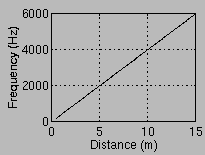 The distance increment
0.1m was chosen arbitrarily. Other values were also tested including
using the resolution of the LRF (0.01m). However, this produced an
increase of 4.38Hz/0.01m which lies within the 'just noticeable difference'
range of 2-5Hz for frequencies between 1000 - 4000Hz. This is the
range required by humans to perceive a change in frequency between pure
tones (Hollander 1994). The graph
on the left illustrates the range of frequencies produced by this mapping.
The distance increment
0.1m was chosen arbitrarily. Other values were also tested including
using the resolution of the LRF (0.01m). However, this produced an
increase of 4.38Hz/0.01m which lies within the 'just noticeable difference'
range of 2-5Hz for frequencies between 1000 - 4000Hz. This is the
range required by humans to perceive a change in frequency between pure
tones (Hollander 1994). The graph
on the left illustrates the range of frequencies produced by this mapping.
4.3.2 INVERSE SQUARE LAW
MAPPING
The decrease of power in sound waves follows the inverse square law (1/distance2).
With several minor changes, this same law was used to map distance to frequency:
-
FREQUENCY = k * ((1/distance2) + c)
-
FREQUENCY = 1333.33 * ((1/distance2) + 0.5)
The constant 'c' (0.5), was used to allow the shifting of the curve to
the right, thereby avoiding any non-audible frequencies (below 20Hz) which
would result with the larger distances. For example, a distance of
12m would be mapped to 9.25Hz without shifting the curve). Allowing
the arbitrary constant c to equal 0.5, the maximum distance is mapped
to 672.60Hz (1333.33 * (1/152 +0.5) = 672.60Hz).
Using the inverse square law was a marked improvement over linear mapping,
however, as shown in table 4.1 of the following page, frequencies changed
drastically for a very small distance range (distances close to the user),
and changed only slightly for the greater distance readings.
|
DISTANCE (m)
|
FREQUENCY (Hz)
|
|
0.50
|
6000.00
|
|
0.70
|
3387.75
|
|
1.00
|
2000.00
|
|
2.00
|
1000.00
|
|
3.00
|
814.81
|
|
10.00
|
680.00
|
|
12.00
|
675.92
|
|
13.00
|
674.58
|
|
14.00
|
673.46
|
|
15.00
|
672.59
|
TABLE 4.1
Inverse square mapping of distance to frequency
As shown in table 4.1 above, the frequency range corresponding to the distances
between 10.00m and 15.00m is insignificant (just above the jnd for frequency
perception). There is no perceived frequency change with a change
in distance above 10.00m and even for distances between 3.00m and 10.00m,
the change in frequency is only 134.81Hz.
Although this mapping was very pleasant to listen to (when distances
were small and a change in frequency could be perceived), it was not used,
largely due to the minimal change in frequency for the farther distances.
Perhaps in the future, this mapping could be used for very close distances,
while another mapping could be used for farther distances.
4.3.3 LOGARITHMIC MAPPING
The following mapping is used to allow for a perceived change in frequency
throughout the entire distance range, and to allow frequency to change
on a logarithmic scale:
FREQUENCY = k * c-(DISTANCE - MIN_DISTANCE) * a
FREQUENCY = 6000Hz * e-(DISTANCE - 0.50m) * 0.15
Subtracting the minimum distance from each distance reading to obtain
the exponent enables the maximum frequency to be used as the frequency
constant. The exponent is then multiplied by a constant ('a'), to increase
the overall frequency for each reading. For example, without this
constant, a distance reading of 10.00m would result in a non-audible frequency
of 0.45Hz, whereas using the constant a = 0.15 results in a frequency of
1443.05Hz. Both constants 'c' and 'a' were arbitrarily chosen.
Various other values of 'c' and 'a' were tested (see figure 4.1 and
4.2 for curves). Using smaller values for 'c' results in a smaller
frequency range (see table 4.3).
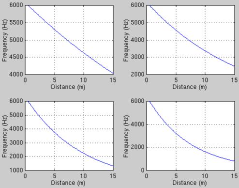
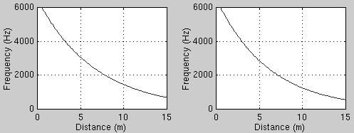 Figure 4.1
Effects of altering the constant 'c' in the formula:
frequency = k * c-(DISTANCE - MIN_DISTANCE) * a
a) frequency = 6000 * 1.2-(DISTANCE
- 0.5) * 0.15 b) frequency = 6000 * 1.5-(DISTANCE
- 0.5) * 0.15
c) frequency = 6000 * 2.0-(DISTANCE
- 0.5) * 0.15 d) frequency = 6000 * 2.5-(DISTANCE - 0.5) *
0.15
e) frequency = 6000 * e-(DISTANCE - 0.5)
* 0.15 f) frequency = 6000 * 3.0-(DISTANCE
- 0.5) * 0.15
Figure 4.1
Effects of altering the constant 'c' in the formula:
frequency = k * c-(DISTANCE - MIN_DISTANCE) * a
a) frequency = 6000 * 1.2-(DISTANCE
- 0.5) * 0.15 b) frequency = 6000 * 1.5-(DISTANCE
- 0.5) * 0.15
c) frequency = 6000 * 2.0-(DISTANCE
- 0.5) * 0.15 d) frequency = 6000 * 2.5-(DISTANCE - 0.5) *
0.15
e) frequency = 6000 * e-(DISTANCE - 0.5)
* 0.15 f) frequency = 6000 * 3.0-(DISTANCE
- 0.5) * 0.15
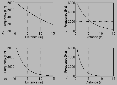 Figure 4.2
Effects of altering the constant 'a' in the formula:
frequency = k * c-(DISTANCE - MIN_DISTANCE) * a
a) frequency = 6000 * e-(DISTANCE -
0.5) * 0.05 b) frequency = 6000 * e-(DISTANCE - 0.5) *
0.2
c) frequency = 6000 * e-(DISTANCE -
0.5) * 0.3 d) frequency = 6000 * e-(DISTANCE - 0.5) * 0.5
Figure 4.2
Effects of altering the constant 'a' in the formula:
frequency = k * c-(DISTANCE - MIN_DISTANCE) * a
a) frequency = 6000 * e-(DISTANCE -
0.5) * 0.05 b) frequency = 6000 * e-(DISTANCE - 0.5) *
0.2
c) frequency = 6000 * e-(DISTANCE -
0.5) * 0.3 d) frequency = 6000 * e-(DISTANCE - 0.5) * 0.5
|
c
|
MIN. FREQ. (Hz)
|
|
1.2
|
4035.82
|
|
1.5
|
2484.00
|
|
2.0
|
1328.65
|
|
2.5
|
817.77
|
|
e
|
681.64
|
|
3.0
|
550.00
|
Table 4.2
Change in the frequency range due to increase
of the constant 'c'.
In each case, the maximum frequency remains 6000Hz
As table 4.3 shows below, using a logarithmic mapping allows a perceived
change in frequency throughout the entire distance range, however, the
changes in frequency were not as drastic as when using the inverse square
mapping for very small distances.
|
DISTANCE
(m)
|
FREQUAENCY (Hz)
|
|
0.50
|
6000.00
|
|
0.70
|
5822.67
|
|
1.00
|
5566.46
|
|
2.00
|
4791.10
|
|
3.00
|
4123.74
|
|
10.00
|
1443.05
|
|
12.00
|
1069.03
|
|
13.00
|
920.13
|
|
14.00
|
791.96
|
|
15.00
|
681.65
|
Table 4.3
Logarithmic mapping of distance to frequency
The logarithmic mapping described above is favoured. In addition
to finding the output tones pleasing, an informal lab survey of three colleagues
found all three preferred the logarithmic mapping over the inverse square
and linear mapping. This version can be found in lrf_main.c along
with its makefile ('makefile').
4.3.4 PIANO KEYBOARD FREQUENCIES
The Sonic PathfinderTM is an ultrasonic travel aid for the visually
impaired, with a maximum range of 8ft divided into eight one-foot sections.
The output consists of the eight notes of the major musical scale (Heyes
1984). Since most people are familiar with the notes of
the musical scale (Heyes, 1980), a practical application
of mapping the distance readings to the 88 keys (52 white keys and 36 black
keys) of the piano keyboard was considered.
As shown below, The frequencies of the piano keyboard range from 27.50Hz
to 4186Hz. This follows the scale of equal temperament in which every octave
(a 2:1 change in frequency), is divided into 12 equal intervals allowing
for the frequency of adjacent notes to differ by a factor of 1.05946 (twelfth
root of two.
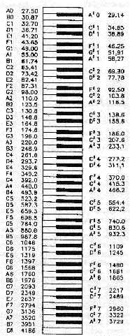 Figure 4.3
Frequencies of the keys on a piano keyboard
Reprinted from "Computer Music" (Jerse,
1985)
Figure 4.3
Frequencies of the keys on a piano keyboard
Reprinted from "Computer Music" (Jerse,
1985)
In order to use this mapping, the frequencies corresponding to the piano
keyboard are stored in a table and mapped linearly to distance. Upon
obtaining a distance reading, the corresponding frequency was looked-up,
the samples were generated and output, (samples were created in real-time).
To determine the appropriate frequency for a distance reading, the following
algorithm is used:
-
Divide the distance range into 88 sections representing the 88 different
frequencies (performed once per program execution only).
-
Divide the distance reading by the above value to obtain table index.
-
Obtain frequency from table (using index determined above).
Figure 4.4 below shows the relationship between distance and frequency
produced by this mapping.
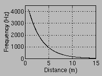 Figure 4.4
Graph of Distance vs. Piano Keyboard Frequencies
Figure 4.4
Graph of Distance vs. Piano Keyboard Frequencies
The output produced by this mapping sounded both very pleasant and realistic.
This was the second mapping used (the first being linear as describe
in section 4.3.1), and appears promising
and is kept separately ('lrf_piano.c'),along
with its own makefile ('makefilePiano'),
allowing for future use and/or modification.
4.4 DISTANCE TO MAGNITUDE
MAPPING
In addition to altering the frequency with distance, altering the
magnitude of the wave inversely with distance was attempted, allowing the
tones corresponding to short distances to sound louder. A magnitude
mapping was included as an option (the mapping is chosen when the constant
definition VARY_MAGNITUDE in lrf_audiov2.h
is defined as any non-zero value). As with the frequency to distance
mapping, several different mappings were tried.
Prior to moving to a PCM encoding, u-law encoding with an 8-bit sample
size was used. This restricted sample sizes to a range of -128 to
127. Along with the problems encountered with scaling the samples
by a value below 0.5 (see
section 4.2), altering the magnitude with distance had a minimal effect
on the output tone. As discussed in section 4.2, the magnitude could
be altered from 0.5 to approximately 2 which is a very small range.
Switching over to PCM allowed a far greater range. In addition
to eliminating the problem of multiplying samples by less than 0.5 (see
section 4.2), the increase in sample size from 8 to 16 meant samples
could range from -32168 to 3276. Altering the magnitude of a wave
is now far more effective.
Using PCM also creates a new problem. Pure tones output appear
to follow the Robinson-Datson "Curve of equal loudness for tones of different
frequencies" (as shown in figure 4.5 below), even when the magnitude of
the wave is not altered.
 Figure 4.5
Robinson-Dadson Curves of Equal Loudness Contours
Figure 4.5
Robinson-Dadson Curves of Equal Loudness Contours
The Robinson-Dadson curve represents the amplitude levels at which single
sine tones of different frequencies sound equally loud. For example,
in order for a 100Hz tone and a 1000Hz tone to sound equally loud, the
amplitude of the lower tone must be boosted by almost 40dB (Moore,
1995). Although the goal was to alter magnitude inversely with
distance, as shown in figure 4.5, the magnitude of a 3500Hz tone exceeds
that of the 6000Hz tone (which represents the closest distance and should
also contain the greatest magnitude), and is definitely perceived so.
This problem can be overcome if the maximum frequency is limited to about
4000Hz. Frequencies increasing from 20Hz up to 4000Hz are perceived
as louder.
4.4.1 INVERSE SQUARE LAW
MAPPING
As in the case of the frequency mapping, this mapping was used to imitate
the reduction in power followed by a sound wave. In this case, however,
it is the magnitude of the wave which is altered as opposed to frequency.
The following formula was used:
MAGNITUDE = k * (1 / distance2)
k = arbitrary constant
Using this mapping it was found that the larger distances are
greatly reduced to the point where they are not audible (when k is less
than about 20). For example, when k = 5, the magnitude corresponding
to 10.00m is 0.05 causing the tone to be barely audible (when k = 0.01,
it results in a non-audible tone regardless the frequency). To overcome
this problem, the value of k can be increased, however, this will also
increase the magnitude of the tones corresponding to the smaller distances
to a point where they are too loud. Extremely loud tones may interfere
with the (possibly important), environmental sounds the user hears (e.g.
passing cars, people etc.).
To decrease the allowable range of magnitudes, several different exponent
values (using the equation above with k=5), were tried as shown in table
4.4 and figure 4.6:
|
EXPONENT VALUE
|
MINIMUM MAGNITUDE
|
MAXIMUM MAGNITUDE
|
|
0.5
|
1.290
|
7.071
|
|
0.7
|
0.751
|
8.122
|
|
1.0
|
0.333
|
10.000
|
|
1.2
|
0.194
|
11.487
|
|
1.5
|
0.086
|
14.142
|
|
2.0
|
0.022
|
20.000
|
Table 4.4
Different exponent values used in the distance
to magnitude mapping: magnitude = k * (1 / distance2)
Max and min magnitude refer to farthest and closest
distance respectively.
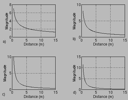
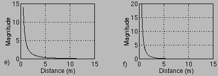 Figure 4.6
Curves produced by altering the exponent in the
formula: magnitude = k * (1 / distanceb)
a) MAGNITUDE = 5 * (1 / distance0.5)
b) MAGNITUDE = 5 * (1 / distance0.7)
c) MAGNITUDE = 5 * (1 / distance1.0)
d) MAGNITUDE = 5 * (1 / distance1.2)
e) MAGNITUDE = 5 * (1 / distance1.5)
f) MAGNITUDE = 5 * (1 / distance2.0)
Figure 4.6
Curves produced by altering the exponent in the
formula: magnitude = k * (1 / distanceb)
a) MAGNITUDE = 5 * (1 / distance0.5)
b) MAGNITUDE = 5 * (1 / distance0.7)
c) MAGNITUDE = 5 * (1 / distance1.0)
d) MAGNITUDE = 5 * (1 / distance1.2)
e) MAGNITUDE = 5 * (1 / distance1.5)
f) MAGNITUDE = 5 * (1 / distance2.0)
An exponent of 0.7 giving a magnitude range of 0.751 to 8.122 was used
(see Table 4.4 above).
4.5 GENERATION OF THE SAMPLES
Regardless of the distance-to-frequency mapping used, the samples representing
the determined frequency cosine wave must be generated. The following
formula is used to generate the samples:
c * ( cos(2 * (f / fs) * n) = sample[n]
c = constant - magnitude scalar of the wave
f = frequency of the cosine wave (in Hz)
fs = sampling rate (in Hz)
n = begins at 0 and is incremented until the final sample is reached
All values generated by the above cosine formula will range between
0 and 1 (this may not be the case when the constant 'c'is greater than
1). Since the audio port requires integer values, these samples are then
converted to the appropriate integer values. The functions provided in
the file 'audio_hdr.h' will
convert the above samples to 8, 16 or 32 bit values.
For each sample the cosine function (cos) is required. In terms
of processor time, the cosine function (available in math.h of the standard
C library), is very expensive, especially when it must be called several
thousand times to create the samples of a single cosine wave. In
an attempt to minimise the time required by the cosine function, a cosine
look-up-table was created. Prior to initiating distance readings,
the cosine values for 100 radian values (increasing by 0.01from 0 to 1.0),
were determined and stored allowing them to be 'looked-up' instead of using
the cosine function. When the cosine of a number is required, the
table is searched for the corresponding cosine value. If found, it
is returned, otherwise, the average of the value below and above are returned.
Quite surprisingly, it actually took longer to use the cosine look-up-table,
as opposed to using the cosine function (see table 4.5). The cosine
function may have its own look-up-table which is more efficient than the
within implementation.
|
RADIAN VALUE
|
TIME
COS FUNCTION
|
TIME
COS TABLE
|
|
0.10
|
12
|
16
|
|
0.25
|
14
|
15
|
|
0.50
|
13
|
16
|
|
0.75
|
14
|
18
|
|
1.00
|
18
|
18
|
Table 4.5
Time required to determine the cosine of a radian
values using the cosine
function compared to using the look-up-table.
The cosine look-up-table was used prior to using a wave-table (see section
4.6), when the samples representing a cosine wave were created upon
receiving a distance reading. Using the wave table, the samples are
created once for the duration of the program prior to initiating the distance
readings. Therefore, even if the cosine-look-up table could be improved
to perform faster than the provided cosine function, the time saved would
be insignificant. Hence, the cosine table is no longer used.
4.5.1 OUTPUT OF A CONTINUOUS
TONE
Irrespective of the distance to frequency mapping used, there is still
a definite amount of time required to obtain a reading. This creates a
break in the output of sound from the time the current tone is heard, to
the time the next tone is heard. In order to allow the perception
of a continuous tone, when a reading is not available from the LRF,
the previous tone is outputted continuously until the next distance reading
becomes available. However, this does not eliminate or decrease the
break between the output of successive tones.
The LRF was set to take 8 readings/second (0.125s/reading). The
time required for the program to obtain a reading, determine the frequency
and generate and output the samples corresponding to this frequency is
0.118s. To allow for a continuous tone the above process must be
accelerated. This prompted creation of a wave-look-up table
(see section
4.6 for a complete explanation), allowing the samples representing
a pre-defined number of frequencies to be stored in a table and used when
needed. With the wave-look-up table in place, the time between the
output of successive tones is greatly reduced allowing the perception
of a continuous tone. Upon obtaining a distance reading from the
LRF, the samples corresponding to it are looked up and continuously output
until the next reading is available from the LRF.
Although a definite change in the pitch of the continuous tone can be
perceived with changing distance, the output of the this tone can become
annoying to the listener after several minutes. In addition, during
the output of frequencies in the range of 3000Hz - 3500Hz, a 'clicking'
sound could be heard in addition to the tone, coming from the background.
This click could be caused from non-matching phase relations of the output
tones. In an attempt to eliminate this problem, outputting one period
only for each wave ensuring correct phase relations was tried. However,
there was no sound at all to be heard when this single period was output.
(It was later found outputting a single period of a tone prevents the tone
from being heard).
Outputting a continuous tone was decided against. In addition
to the 'click' problem described above, after several minutes, the sound
was bothersome to the listener.
This version was also kept separately (lrf_main2.c), along with its
makefile (makefile2).
4.6 REAL-TIME
SAMPLE GENERATION vs. WAVE-TABLE LOOK-UP
The samples corresponding to each cosine wave can be generated immediately
upon receiving a distance reading from the LRF (real-time), or the samples
can be calculated and stored in a wave look-up-table (a pre-defined number
of frequencies will be created), prior to initiating readings from the
LRF. In this case, when a reading is obtained, the samples corresponding
to it are 'looked-up' and output.
Using real-time generation allows the mapping of each distance to a
unique frequency cosine wave, whereas when using the table of samples,
certain distances will respond to the same frequency output. However,
the difference between the frequencies decreases as the distances increase,
(using the present logarithmic mapping), and since humans require a minimum
change of frequency between two pure tones (about 2-5 Hz), to perceive
them as different (Hollander, 1994), the real
time generation is not essential.
Real-time generation is approximated using the look-up-table by increasing
the number of frequencies stored in the table. However, increasing
the number of frequencies stored causes an increase in both the memory
space required, as well as the time to initialise the table.
A look-up-table containing samples for 145 cosine waves was used.
This table contains waves for distances ranging from MIN_DISTANCE (0.5m)
increasing by 0.10m until MAX_DISTANCE (15m). The increment of 0.10m
represents the accuracy of the LRF (see section
2.3.1.7).
With the present size table, it takes approximately 8 seconds to initialise.
Nevertheless, time is saved using the look-up-table. In particular,
it takes approximately 0.091 seconds to obtain a reading, determine and
output the corresponding samples whereas using real-time sample generation
takes approximately 0.118 seconds (see section
3.9.3 for the time determination). This decrease in operation
time allows for an increase in the number of readings taken per second
(shots/reading was changed from 150 to 120 as a result).
4.7 DEPTH DISCONTINUITY (DC)
There are many situations where the difference between the present distance
reading and the previous distance reading is large (larger than a pre-defined
value 'DEPTH_DISCONTINUITY' as defined in lrf_audiov2.h).
This is defined as a depth discontinuity, or, a sudden change in
depth. It is important to convey such information to the user.
For example, this could be used to locate a doorway with the door open
since the distance to the object beyond the doorway (a wall etc.) will
generally constitute a depth discontinuity.
Distance changes greater than 1.50m will result in a depth discontinuity.
It was found that using a value greater than this will prevent several
instances where there is a depth discontinuity from being conveyed to the
user. For example, by measuring the distance between several doorways and
the wall beyond, there were several instances where the depth discontinuity
is quite small (e.g. less than 2.0m), as shown in table 4.6 below:
|
DOORWAY
|
DISTANCE TO WALL (m)
|
|
door in my room (in my house), to hallway wall
|
1.3
|
|
VGR lab to hallway lab
|
2.1
|
|
door in my sister's room to hallway
|
2.6
|
|
door in my brother's kitchen to hallway wall
|
1.5
|
Table 4.6
Distance difference between a doorway and the
wall beyond.
To convey a depth discontinuity to the user, a signal different from any
of the pure tones used for regular output was used, ensuring that a depth
discontinuity corresponded to a unique signal. Initially, a pure
tone of a frequency not used in the regular distance to frequency
mapping was applied. Experimentation with various low frequency tones
(100Hz, 200Hz, 300Hz etc.) was conducted since for all frequency mappings
used, the minimum frequency used was about 600Hz. Although the low
frequencies (below 300Hz), sounded differently, they did not seem
to grab the user's attention, as they were still pure tones. Moreover,
unless someone is really familiar to the tones output, it could easily
be confused with a tone corresponding to a large distance. (This
was the case with one person who used the unit for several minutes with
no prior use and only a brief description of its use). Several other
signals were created as described below:
4.7.1 SUMMATION OF SINE WAVES
As proven by Jean Baptiste Fourier, every periodic waveform is comprised
of a unique set of sinusoids whose frequencies are harmonically related.
Thus any waveform can also be described in terms of the sinusoidal components
that it contains (Jerse 1985).
To achieve this summation effect with sampled waveforms, the following
formula is used for each sample:
sumWave[n] = k1 * cos(2 * PI * (f1
/fs) * n) + k2 *cos(2 * PI * (f2 / fs)
* n) + ki cos(2* PI * (f3 / fs)
* n)
Using the above formula, several combinations of cosine waves were summed
with the resulting wave used as a depth discontinuity signal. Initially,
summing non-harmonic waves was yielding a sound not much different from
the pure tones used.
The next method used was approximating a square wave (whose spectrum
contains an infinite number of odd harmonics of the fundamental whose amplitudes
decrease in proportion to the increasing harmonic number). Although
an infinite number of samples could not be used, using about seven
allows a square wave to be approximated. The following formula was
used:
sumWave[n] = k1 * cos(2 * PI * (f1
/ fs) * n) + k1 / 3 *cos(2 * PI * (3f1 /
fs) * n) + ? + ki/ 7 *cos(2 * PI * (7f1
/ fs) * n)
k1 = 5
f1 = 200Hz
Using a square wave did not produce a change over the previous signal
containing non-related harmonics.
4.7.2 TRIANGULAR AND PULSE
SIGNALS
Although using a summation of tones is an improvement over using a single
tone to convey a depth discontinuity, it still does not have the effect
of 'grabbing' the listener's attention. Producing a short pulse
or single triangular signal in an attempt to create a sudden 'bang' was
attempted.
To create the samples representing the pulse, values representing PCM
encoding (-32768 to 32767), were assigned directly to the samples in the
following manner:
-
Assign a value to the first sample (a smaller value, for example -32768
or 0)
-
The remaining N-1 samples are assigned the same value (much larger than
the first, for example 32767).
-
The last sample is assigned the same value as the first sample.
Regardless of the values used, as long as there was a substantial increase
in the samples following the first) the pulse sounded the same. For
example, assigning the same value between -32768 and 0 to the first
and last sample and 32768 to the samples in between produced the
same effect.
To create a single triangular signal, several different methods were
used, as described below:
4.7.2.1
PROBABILITY: THE TRIANGULAR DISTRIBUTION:
The book Computer Music by Doage Jerse contains
various algorithms for generating several random and probability
processes. It includes the triangular distribution which can generated
by assigning to each sample the average of two randomly generated values.
The random number generator available in the C-library generates values
between -32768 and 32767, the same range required by the samples.
This method was used with several different amounts of samples (60,
100, 200, 500, 1000), however, in all cases, the only output produced was
noise. Upon examining the samples, they did not appear to have a
triangular distribution but rather were scattered (e.g. the samples did
not begin to increase until a maximum point was reached, then decrease
back to the starting point).
4.7.2.2 TRIANGULAR FORMULA:
The following formula was used to generate the samples representing the
first half of the triangular wave:
sample[i] = c * n * t
c = constant
t = Sample rate period * number of samples (duration of the
signal)
n = ranges from 0 increasing by 1, to 15 the total number of samples
To create the second half of the wave, n was then decreased until it
became zero.
The following algorithm was used to implement the above function:
-
Determine the wave duration by multiplying the total number of
samples by the Sampling Period (time taken to take one sample).
-
Determine the value of the constant 'c' by assigning an arbitrary value
to sample[n] (representing the peak of the triangle) and solving the equation
for 'c'.
-
Using the value for 'c' obtained above, solve the equation for all samples
ranging from 0 to 15 the total number of samples.
Several different peak values were used and, in each case, examining
the samples confirmed the triangular pattern. There was an increase
in sample values beginning with the first sample until half way through,
where the maximum value was encountered. The remaining samples then
decreased until they reached the minimum value once more. Irrespective
of the peak value used, a change in the output signal was imperceptible.
NOTE:
While experimenting with the triangular and pulse signals, using the
u-law encoding, I found
that sending less than nine samples to the audio port resulted in a
'click' being output regardless of the value of the samples. Sending
over nine samples resulted in no sound heard. I could not understand
this effect as the duration of nine samples is far less than the minimum
duration required to perceive a sound.
When sending data to any port using the write system call, the number
of bytes to write must also be specified. It took several hours to
realise I was sending nine bytes and specifying 4000 bytes were being sent!
The pulse and triangular signals were clearly distinguishable from
any of the pure tones or pure tone summations used previously. Yet, they
both sounded the same, having very short durations and weak signals, making
them barely audible. In order to overcome this problem, the signal
was output continuously for a set number of times. By outputting
the pulse, triangular signals or pure tones in loop a certain number of
times, gives the effect of a continuous signal, with no breaks in between.
As table 4.8 below shows, both signals took about the same amount of time
to produce and output.
|
NUMBER OF SAMPLES
|
TIME FOR PULSE (s)
|
TIME FOR TRIANGLE (s)
|
|
60
|
0.001
|
0.001
|
|
100
|
0.002
|
0.003
|
|
200
|
0.006
|
0.007
|
Table 4.8
Time to generate and output the triangular and
pulse signals
For both triangular and pulse signals, generating and outputting less
than about 20 samples, results in a non-audible signal. Furthermore, as
the number of samples are increased beyond 200, the signal begins to sound
like noise. Since both signals sound the same, currently the
pulse signal is used to convey a depth discontinuity since it is easier
to implement.
4.7.3
USING AN AVERAGE OF THE N PREVIOUS DISTANCES
Comparing the current reading to the previous reading to determine whether
a depth discontinuity has been encountered, apparently is effective.
However, in an attempt to limit the possibility of errors due to LRF reading
resolution etc. the current distance reading was compared to the average
of the previous N readings (values for N tried were 5, 10, 15). To
achieve this, the following algorithm was used:
-
Obtain distance reading.
-
Calculate average of the previous N readings.
-
Compare the current distance reading with average of previous N readings.
-
Replace oldest distance of previous readings with the current reading.
-
Determine how many previous readings exist.
Although the number of previous readings was pre-defined, a check
is required to determine how many previous distances exist in order to
calculate the average, given that the program initially begins with
0 previous distances (when the first distance reading is obtained).
Instead of limiting the possibility of errors, it was found that
an average actually created errors in several circumstances, when a depth
discontinuity, although existing, was not detected. For example,
consider N = 5 and the following five previous distances:
0.80, 0.75, 0.95, 0.92, 0.5
with the current distance reading of 2.10m. The average of the
above five readings is 0.784. Using the current distance difference
required for a depth discontinuity (1.5m), there is clearly a depth discontinuity
between the last of the readings (0.50m) and the current reading (2.1m).
However, using the average of the above five readings (0.78m), does not
result in a depth discontinuity
(2.10m - 0.78m = 1.32m).
Regardless of the value used to compare depth discontinuities, examples
of the foregoing can be easily found. As a result, averaging
the previous N readings was not used. The function calcAverage()
(see 'lrf_audiov2.c'), was used to calculate
the previous readings. Although it is presently not used, it is included
in the event of future applications.
5. INTERNET SITES VISITED
5.1 RELATED RESEARCH
(PAST AND PRESENT)
Below are sites related to research conducted (both past and present),
related to Mobility Aids, Electronic Travel Aids, Auditory Displays, Auditory
Scene Analyses etc. Any products mentioned are not available commercially
(yet).
1. http://www.psyc.nott.ac.uk/bmru/history.html
History of the Blind Mobility research Unit from 1965-1995 at Nottingham
University. Describes the development of Electronic Travel Aids,
mobility for the blind in general and the involvement of the above research
unit in the field.
2. http://www.ul.cs.cmu.edu/books/mobility_aids
ELECTRONIC TRAVEL AIDS: NEW DIRECTIONS FOR RESEARCH. A 124 page
publication from the Working Group on Mobility Aids for the Visually Impaired
and Blind. Committee on Vision. National Research Council.
The following topics are covered:
-
The Demography of Blind and Visually Impaired Pedestrians
-
Assessment of Mobility
-
Perceptual, Cognitive, and Environmental Factors
-
Sensory Enhancement and Substitution
-
The Technology of Electronic Travel Aids
3. http://www.robots.ox.ac.uk:5000/~pjp/rank.html
"Rank Prize Fund Meeting: Technology to Assist the blind
and Visually Impaired". A conference held in the UK March 25-28
1996 of the There are no complete papers available however, abstracts describing
several topics including navigation and mobility for the blind, are available.
5.1.1 OBSTACLE DETECTORS
Warn only of the presence and possibly a distance to the object in the
user?s path.
1.
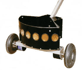
http://bme01.engr.latech.edu/cdrom/texts/321.html
DYNAMIC ULTRASONIC RANGING SYSTEM (~1993/94):
-
A prototype built around a PVC tube resembling a long cane.
-
Four computer controlled ultrasonic sensors provide real-time information
on distance and height within 5m of the user.
5.1.2 ORIENTATION
AND NAVIGATIONAL AIDS
Convey information to the user regarding the geographical area (orientation)
and help the user find their way from location A to location B (navigation).
1. http://simsrv.cs.uni-magdeburg.de/~mobic/tideful.html
MoBIC (MOBILITY OF BLIND AND ELDERLY PEOPLE INTERACTING WITH COMPUTERS)
(1995):
-
Does not provide obstacle detection.
-
Orientation and navigation aid through the use of GPS.
-
Consists of two parts:
1. MoPS (Mobile Pre-Journey System):
-
helps a user plan a journey (obtains map information, bus/train schedules
etc.).
-
provides data specific to the blind traveller.
2. MoODS (Mobile Outdoor System):
-
Guides the user towards their destination using GPS and an electronic
compass
-
User can ask certain questions, for example "where am I", through a
hand held keyboard.
2. http://www.cs.tcd.ie/PAMAID
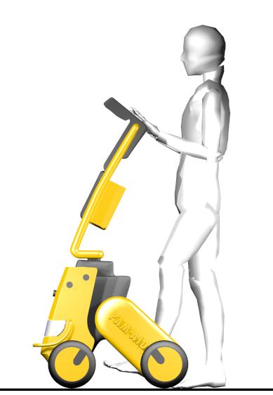 PAM-AID (PAERSONAL
ADAPTIVE MOBILITY FOR FRAIL AND ELDERLY BLIND PEOPLE); TELEMATICS APPLICATION
PROGRAM (JAN. 97 - PRESENT):
PAM-AID (PAERSONAL
ADAPTIVE MOBILITY FOR FRAIL AND ELDERLY BLIND PEOPLE); TELEMATICS APPLICATION
PROGRAM (JAN. 97 - PRESENT):
-
Uses technology from industrial automation.
-
The objective of PAM-AID is to allow users to retain their personal
autonomy.
-
Supports three modes of operation:
1. HUMAN CONTROL:
-
Issues warnings when an obstacle is detected and intervenes if there
is severe danger.
2. UNSUPERVISED CONTROL:
-
the system navigates unsupervised avoiding obstacles.
3. SHARED CONTROL:
-
system makes small adjustments to minimise the risk of a collision.
3. http://phenix.herts.ac.uk/PsyDocs/sdru/index.html
University of Hertfordshire Sensory Disabilities Research unit.
Includes information regarding the following projects:
-
MoBIC (project member)
-
GUIB (Graphical User Interface for the Blind)
-
PAM-AID (project member)
4. http://www.cs.tcd.ie/gjlacey
Home page of Gerrad Lacey, a Computer Science graduate student at Trinity
College Dublin, Dublin Ireland. His research interests include "The
application of mobile robot technology to the mobility of the frail visually
impaired". Several of his publications are available online including
"Personal Adaptive Mobility Aid (Pam-AID) for the Infirm and Elderly Blind",
"Autonomous Guide for the Blind' and "Evaluation of Robot Mobility Aid
for the Elderly Blind".
5. HTTP://www.engin.umich.edu/research/mrl/00MoRob_22.html
GUIDECANE
(Guidance Device for the Blind)
-
An array of ultrasonic obstacle-sensors attached to a wheeled handle
or cane.
-
The user selects a direction of travel by using a joystick on the cane
and then pushes the cane forward. The user can then turn right
or left moving the joystick in the respective location.
-
When the sensors detect an obstacle, the best path around the obstacle
is determined and the wheeels are turned accordingly. Through the
cane the user feels the change of direction and follows. Once the
obstacle is passed, the cane brings the user back to the desired direction
of travel
-
Uses an on-board 25MHz 486 PC.
-
Weighs only 4kg.
-
Contains 10 ultrasonic sensors capable of sensing any obstacles within
120o.
Part of the above description was reprinted from IEEE Spectrum October
1997.
6. HTTP://www.arkenstone.org/
STRIDER - A Talking Portable Navigation System: (by Arkenstone)
-
Addresses the transportation needs of the visually impaired.
-
Consists of a Global Positioning System (GPS) and Differential GPS receivers
which plug into a notebook computer.
-
The GPS receivers provide lthe system with the user's latitude and longitude
positions which after processing, the location of the user is conveyed
to the user through software speech.
-
Currently a proto-type (packaged in a backpack), has been developped.
5.1.3 ENVIRONMENTAL AIDS
Detect object(s) but also provide characteristic information about the
object(s) and possibly the environment as well.
1. http://ourworld.compuserve.com/homepages/Peter_Meijer
vOICe (1994):
-
Converts images taken with a standard T.V. camera into sound patterns
on a 1-1 image to sound mapping ensuring preservation of the visual information
(Meijer, 1992).
-
Each picture is sub-divided into 4096 pixels (64*64) and each pixel
can be one of 16 shades of grey.
-
Every column is then translated into a sound (top pixel is high pitched,
bottom pixel is low pitched and intermediate pixel has intermediate pitch.
The shade of the pixel indicates the loudness), and then summed allowing
them to be heard simultaneously.
-
The visual image is scanned from left to right outputting the sound
of each column.
-
Pictures are taken and converted to sound every second.
-
Real-time processing.
2. http://zadok.eeng.dcu.ie:800/~mollyd/docs/spie/spie.paper.html
"APPLICATION OF MACHINE VISION TECHNOLOGY TO THE DEVELOPMENT OF AIDS
FOR THE VISUALLY IMPAIRED": Dublin University, School of Electrical
Engineering.
-
Combination of shape, colour and motion is used to provide an auditory
description of an image obtained through a camera linked to the Prolog
environment.
1.
Shapes: Identified by obtaining certain characteristics and
then comparing them against
reference characteristics. Described using synthesised
voice output.
2. Colour: Tone of sound is mapped to hue, loudness is
mapped to brightness.
2. Motion: Centroid Tracking and Motion Tracking are
separately experimented.
3. http://ourworld.compuserve.com/homepages/Vuphonics
VUPHONICS (86 - PRESENT):
-
Sound (coded phonetics, multiple voices), resembling a language (English
of European), which the user recognises and assigns meaning to, leading
to a mental image, are output.
-
Factual information (e.g. colour), is also conveyed by sound.
-
The user builds up the layout of a scene on a rectangular grid where
the resolution varies (resolution increases near areas of attention).
-
Images to be conveyed are stored as the sections of a grid and sounds
representing the overall light characteristics of and relative distances
of features in the sections of images are output in a structured manner.
5.1.4 VIRTUAL SOUND:
1. http://www.hitl.washington.edu/publications/hollander/home.html
AN EXPLORATION OF VIRTUAL AUDITORY SHAPE PERCEPTION:
Master's thesis of Ari J. Hollander exploring
the potential to perform shape recognition of virtual auditory objects.
Contains a very good summary of auditory perception and mentions many previously
conducted experiments.
5.2 Commercial Products
The sites below refer to Electronic Travel Aids presently (and previously),
available commercially.
1. http://www.sonicvision.co.nz
Sonic Vision - a company of Leslie Kay (a pioneer in the Electronic
Travel Aid field). Site contains information and diagrams of the
following three products:
 BINAURAL SENSORY
AID (SONICGUIDE) (1965):
BINAURAL SENSORY
AID (SONICGUIDE) (1965):
-
Environmental Aid.
-
Pair of glasses containing an ultrasound emitter and two receivers (left,
right), whose signals are fedseparately to the corresponding ear allowing
for object location to be determined through binaural hearing.
-
Distance up to 18ft.,is indicated inversely with pitch (higher pitch
= greater distance).
-
Quality of the output sound can be used to identify object surface (clear
sound = hard surface, fuzzy sound = rough surface).
-
Does not interfere with normal hearing.
-
Can be used to teach perceptual development to blind infants and children.
-
Does not detect drop-offs, curbs.
 TRISENSOR (KASPA)
(1994):
TRISENSOR (KASPA)
(1994):
-
SonicguideTM mounted on a head band, with an added high resolution
monaural sensor in order to model the dual function of the eye (fovial
and peripheral fields of view).
-
Uses a micro-processor to generate high resolution location of objects.
-
Location of multiple objects in a 90o field of view.
2. http://ariel.ucs.unimelb.edu.au/~heyes
Tony Heyes' Perceptual Alternatives home page containing information
about the Sonic Pathfinder. Links to other sites related to blind
mobility are also available.
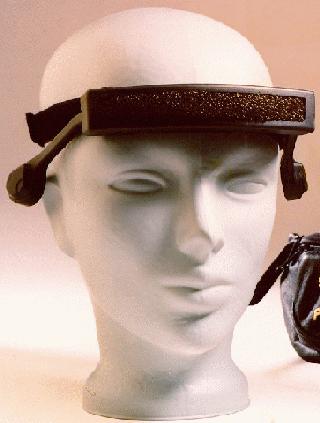 SONIC PATHFINDER:
-
Environmental Aid with a range of about 8ft.
-
Head mounted computer controlled sonar system containing three receivers.
-
Notes of the musical scale are output progressing in tone as the object
is approached.
-
Object to the left or right of the user causes the tone to be heard
in the respective ear whereas an object directly ahead outputs the tone
to both ears.
-
The presence of the nearest object is conveyed and without any object
present, the user is informed about the proximity of the shore-line.
5.3 MIDI SITES
http://www.harmony-central.com/MIDI/Doc/tutorial.html
Complete MIDI tutorial including diagrams/pictures covering the following
topics:
-
MIDI vs. Digitised Audio
-
MIDI Basics
-
MIDI Messages
-
Synthesiser Basics
-
PC to MIDI Connection
-
MS Windows Configuration
2. http://www.borg.com/~jglatt/tutr/miditutr.html
"Documents that explain MIDI concepts in non-technical terminology.
Also contains information that may be useful to musicians using MIDI based
products." Some of the topics covered include:
-
Basic Tutorial
-
Hardware Discussions
-
Computer and Hardware Configuration/Setup/Troubleshooting
-
Performance and Sequence Tips
-
Useful Charts
3. http://www.borg.com/~jglatt/tech/miditech.html
Technical details of MIDI (including General MIDI, MIDI file format,
MIDI sample dump standard, MIDI time code), as well as MIDI programming
information.
5.4 MISCELLANEOUS SITES
1. http://www.santafe.ed/~icad
ICAD (International Conference on Auditory Displays). Contains
conference proceedings for 1992/94/96, links to journals related to auditory
research and perception.
2. http://sound.media.mit.edu/AUDITORY/asamtgs
Abstracts from the Acoustical Society of America conferences (124-130th
meetings). Many topics related to auditory perception, auditory scene
analysis psychoacoustics etc.
3. http://www.rnib.org.uk
Home page of the Royal National Institute for the Blind (UK) containing
general information on blindness and the needs of the blind. Contains
many links to other sites.
4. http://www.psych.not.ac.uk/bmru
Nottingham University, Department of Psychology, Blind Mobility research
Unit. Includes information describing their current:
NOMAD: Purpose of the project is to help visually impaired students
find their way on campus
through the use of an audio and tactile graphics map of the campus.
5. http://www.robots.ox.ac.uk/~david/home.html
Home page of David Lee (member of the Robotics Research Group.).
Several papers related to the mobility of the blind are available including
"Object recognition with FM Sonar".
5.4.1 LINKS TO OTHER RELATED
SITES
1. http://www.nyise/research.html
New York Institute for Special Education. Contains links to blindness
related sites.
2. http://www.cs.yorku.ca/~billk
Summary of some of the work conducted in the field of Electronic Travel
Aids. Includes a description of many products (both past and present).
Some of the information on this site appears in this report.
3. http://datura.cerl.uiuc/netstuff/sigSoundLinks.html
Many links to sites related to the following:
-
Auditory Research
-
Computer Music
-
Sonification and Virtual Environment
-
Speech
-
DSP
-
Hyper Audio
4. http://www.aber.ac.uk/~dgw/3daudio.htm#Reasearch
"Links to 3D and spatial sound related resources on the web. Reference,
research, educational tools, people, commercial systems and products.
Links to other 3D related and general audio lists and patent resources".
5.5 NEWSGROUPS
On several occasions questions regarding problems encountered with equipment,
programming etc. were posted to the appropriate newsgroup(s).
comp.music.research
comp.music.dsp
comp.music.midi
comp.sys.sun.hardware
comp.sys.sun.misc
comp.lang.c
6. SUGGESTIONS AND CONCLUSIONS
6.1 IDEAS
FOR FUTURE CONTINUATION OF THE PROJECT
6.1.1 USE OF MIDI TO
GENERATE SOUND
As suggested by Professor Dymond, instead of generating and outputting
pure tones, MIDI could be used to produce a wide range of sounds, including
the sound of musical instruments to be output. For example,
a drum bang can easily be output when a depth discontinuity is encountered
instead of outputting the current pulse signal.
6.1.2
USE OF A MACINTOSH COMPUTER OVER THE SUN WORKSTATION
The SUN workstation is fairly limited in terms of its audio capabilities.
For example, it does not support MIDI. Also, the SUN is not portable,
hence, any experimentation is restricted to workstation room (i.e. one
cannot perform any mobility tasks using the device blindfolded outdoors).
In addition to supporting MIDI (both hardware and software), being
portable, and its quality sound output, there is a great deal of sound
related software available for the Macintosh making it the choice for many
musicians and sound researchers. Any future work on this project involve
switching computer platforms to the Macintosh.
6.1.3
ELIMINATING THE EFFECTS OF THE ?CURVE OF EQUAL LOUDNESS?
As discussed in section 4.4, the magnitude of the pure tones output followed
the "Curve of Equal Loudness" (Robinson-Datson curve, figure
4.5) in which tones of different intensity levels are perceived to
have the same loudness. Currently a 3.5kHz tone associated with a
distance of 3.5m sounds louder than a 6kHz tone associated with a distance
of 0.5m even though shorter distances are supposed to be mapped to louder
sounds. A function could be created to eliminate the effect of the
Robinson-Datson curve. This would allow all frequencies to be perceived
at the same magnitude thereby giving the user the choice of altering
the magnitude or not.
6.1.4 EXPERIMENTATION
With the use of a portable computer, blindfolded or visually impaired persons
could use the device while performing simple mobility tasks (e.g. walking
outdoors etc.) in order to determine the effectiveness of the device as
a mobility aid.
6.1.5 NEW 'POWER' AND 'DATA OUT' CONNECTORS REQUIRED
As discussed in section 2, the 'POWER' and 'DATA
OUT' connectors to the LRF must be replaced because they contain loose
connections which occasionally result in the loss of power to the LRF as
well as the loss of data to the remote terminal via the serial connection.
6.2 CONCLUSIONS
I have learned much about serial communications, audio generation using
the SUN workstation, the perception of sound by humans and Electronic Travel
Aids. In addition, the information gathered and the software written
during this four month period will serve as a framework for any continuation
on this project. Although extensive testing was not carried out due to
hardware limitations and lack of time, I believe the project was successful.
6.3 Acknowledgements:
I would like to thank Professor Milios and Greg Reid for their help with
many of the problems I encountered while working on this project. I would
also like to thank Antonin Pribetic and Nancy Kapralos for taking time
off their busy schedule to proof-read my final report.
7. REFERENCES
7.1 BIBLIOGRAPHY
Aitken, Stuart and T. G. R. Bower. (1982). "Intersensory Substitution in
the Blind." Journal of
Experimental Child Psychology. 8 1275.
Arias C. C. A Curet. H. F Moyano. S. Joekes and N.
Blanch. (1993). ?Echolocation: A study of
Auditory Functioning in Blind and Sighted
Subjects.? Journal of Visual Impairment and Blindness,
87, 73-77.
Blasch, B B. G. Lang and N. Griffin-Shirley. (1989). "Results
of a National Survey of Electronic
Travel Aid Use." Journal of Visual Impairment
and Blindness, 83, 449-453.
Bower, T. G. R. (1982). "The Use of SonicguideTM in Infancy." Journal
of Visual Impairment and
Blindness, 76, 91-100.
Brabyn, John. (1982). "Problems to be Overcome in High-Tech
Devices for the Visually Impaired."
Optometry and Vision Science, 69 (1), 42-45.
Brabyn, John. (1985). "Development in Electronic Aids for
the Blind and Visually Impaired." IEEE
Engineering in Medicine and Biology Magazine,
December 1985, 33-37.
Bregman, A. S. (1990). Auditory Scene Analysis: The Perceptual
Organisation of Sound. MIT Press,
Massachusetts, U.S.A.
Buser, P and M. Imbert. (1992). Audition. MIT Press, Massachusetts,
U.S.A.
Crispien, Kai and Klaus Fellbaum. (1996). "A 3-D Auditory
Environment for Hierarchical Navigation
in Non-visual Interaction." Proceedings
of ICAD 1996.
Dodds, G. Allan. (1983). "The Sonic Pathfinder - an
Objective Evaluation." International Journal of
Rehabilitation Research, 6 (3), 350-351.
Dodds, G. Allen, J. D. Armstrong and C. A. Shingledecker.
(1981). "The Nottingham Obstacle
Detector: Development and Evaluation."
Journal of Visual Impairment and Blindness, 75, 203-209.
Dodge, Charles and Thomas A. Jerse. (1985). Computer
Music, 2nd Edition. Schrimer Books, New
York, U.S.A.
Easton, D. Randolph. (1992): "Inherent Problems of Attempts
to Apply Sonar and Vibrotactile
Sensory Aid Technology to the Perceptual Needs
of the Blind." Optometry and Vision Science 69
(1), 3-14.
Fish, M. Raymond and Ronald C. Fish. (1976). "An Electronically Generated
Audio Display for the
Blind." Journal of Visual Impairment and Blindness,
70, 295-298.
Frisken-Gibson F. Sarah, Paul Bach-Y-Rita, Willis J. Tompkins and John
G. Webster. (1987). "A
64-Solenoid, Four Level Fingertip Search Display
for the Blind." IEEE Transactions on
Biomedical Engineering, 34 (12), 963-965.
Frysinger, P. Steven and Gregory Kramer, (eds) (1996). Proceedings of
the Third International
Conference of Auditory Display, held November
4-6, 1996, Palo Alto California.
Gao, X. Robert and Li Chuan (1993). "A Dynamic Ultrasonic Ranging
System as a Mobility Aid for
the Blind." Louisiana Technical University.
Ruston (U.S.A).
Guarniero, Gerard. (1977). "Tactile Vision: A Personal
View." Journal of Visual Impairment and
Blindness, 71, 125-131.
Heyes, D. Anthony. (1990). "The Sonic Pathfinder."
TechniTalk, Winter 1990.
Heyes, D. Anthony. (1984). "The Sonic Pathfinder: A New Electronic
Travel Aid." Journal of Visual
Impairment and Blindness, 77, 200-202.
Hioki, Warren. (1990). Telecommunications. Prentice
Hall, New Jersey, U.S.A.
Hollander, A. J. (1994). "An Exploration
of Virtual Auditory Shape Perception." Ph.D.thesis,
human Interface Technology Lab, University
of Washington, U.S.A.
Kao, Gordon, Penny Probert and David Lee. (1996) "Object Recognition
with FM Sonar: An Assistive
Device for Blind and Visually Impaired People."
American Association for Artificial Intelligence.
Kay, Leslie. (1980). "The Sonicguide, Long Cane and Dog
Guide: Their Compatibility." Journal of
Visual Impairment and Blindness, 74, 277-280.
Kay, Leslie. (1984). "Acoustic Coupling to the Ears in Binaural
Sensory Aids." Journal of Visual
Impairment and Blindness, 77, 12-16.
Kendall, S Gary. (1991). "Visualisation by Ear: Auditory
Imagery for Scientific Visualisation and
Virtual Reality." Computer Music Journal,
15, (4) 70-73.
Koren (Dr.). (1995). Course Notes: Protocols &
Computer Networks. Tel-Aviv
University. (http://www.rad.com/networks/1995/rs232/rs232.html)
Kramer, Gregory and Stuart Smith, (eds) (1994). Proceedings of the Second
International Conference
on Auditory Display, ICAD '94, held
November 7-9, 1994, Santa Fe, New Mexico.
Lacey, Gerrard and Kenneth Dawson-Howe. (1997). "Evaluation of Robot
Mobility Aid for the Elderly
Blind." Proceedings of the Fifth International
Symposium on Intelligent Robotic Systems,
Stockholm Sweden.
Lacey, Gerrad and Kenneth Dawson-Howe. (1997). "Personal
Adaptive Mobility Aid (PAM-AID)
for the Infirm and Elderly Blind." Lecture
Notes in AI: Assistive Technology & Artificial
Intelligence. Mittal Vibhu, Holly Yanco
and John Aronis. (eds).
Loomis, M. Jack, Chick Hebert and Joseph G. Cicinelli. (1990).
"Active Localisation of Virtual
Sounds." The Journal of the Acoustical
Society of America, 88 (4), 1758-1764.
Loomis, M. Jack, Roberta L. Klatzky, Reginald G. Golledge, Joseph
G. Cicinelli, James W Pellegrino
and Phyllis A. Fry. (1993).
"Nonvisual Navigation by Blind and Sighted: Assessment of Path
Integration Ability." Journal of Experimental
Psychology: General, 122 (1), 73-91.
Loomis, M. Jack, Reginald G. Golledge, Robert L. Klatzky, Jon M. Speigle
and Jerome Tietz. (1994).
"Personal Guidance System for the Visually
Impaired." Department of Psychology, University of
California.
McKennell, A. Bruce and E. Walker. Blind and Partially Sighted
Adults in Britain: The RNIB Survey.
Volume 1, Her Majesty?s Stationary Office,
London.
Meijer P.B.L. (1992). "An Experimental System for Auditory Image
Representation.". IEEE
Transactions on Biomedical Engineering,
39 (2), 112-121.
Miletic, G. (1994). "Vibrotactile Perception: Perspective
Taking by Children who are Visually
Impaired." Journal of Visual Impairment
and Blindness, 88, 550-551.
Miletic, G, B. Hughes and Paul Bach-y-Rita. (1988). "Vibrotactile Stimulation:
An Educational
Program for Spatial Concept Development."
Journal of Visual Impairment and Blindness, 88,
366-370.
Miller, L. (1992). "Diderot Reconsidered: Visual Impairment
and Auditory Compensation." Journal
of Visual Impairment and Blindness, 86, 206-210.
Mims M. Forrest. (1973). "Sensory Aids for Blind Persons." The New Outlook,
November 1973, 67,
407- 414.
Molly, D, T. McGowan, K. Clarke, C. McCorkell and P. F. Whelan. (1994).
"Application of Machine
Technology to the Development of Aids for
the Visually Impaired." Proceedings Machine Vision
Applications, Architectures and Systems Integration.
Oct. 31 - Nov. 2 1994, Boston U.S.A.
Moore, C. J. Brian, (ed) (1995). Hearing. Academic
Press, San Diego California, U.S.A.
Moravesik, J. Michael. (1987). Musical Sound: An Introduction
to the Physics of Computer Music.
Solomon Press, U.S.A.
Moricca, S. Larry and Rex V. Slocum. (1977). "Pattern recognition
on the Forehead: An Electronic
Scan System." Journal of Visual Impairment
and Blindness, 71, 164-167.
Paturzo, Anthony Bonaventura. (1984). Making Music with MicroProcessors.
Tab Books, Philadelphia
U.S.A.
Plomp, R. (1976). Aspects of Tone Sensation. Academic Press, New York,
NY, U.S.A.
Pohlmann, C. Ken. (1989). Principles of Digital Audio, 2nd Edition.
Howard W. Sams & Company,
U.S.A.
Pollack, Irwin and Mitchel Rose, (1967). "Effect of Head Movement on
the Localisation of Sounds in
the Equatorial Plane." Perception and Psychophysics
Rossing, D. Thomas. (1982). The Science of Sound. Addison-Wesley Publishing
Company, U.S.A.
Rothstein, Joseph. (1995). MIDI: A Comprehensive Introduction.
Maddison Wesley Publishers, U.S.A.
Scadden, Lawrence. (1969). "A Tactual Substitute for Sight." New
Scientist. 41, 677-678.
Schustermann, J. Ronald. (1965). "Echo Detection Ability of the Blind:
Size-Distance Factors."
Journal of Experimental Psychology. 70, 245-251.
Scione, M. W (1978). "Electronic Sensory Aids in a Concept Development
Program for Congenitally
Blind Young Adults." Journal of Visual
Impairment and Blindness, 72, 88.
Simon, Permina Ellen. (1984). "A Report on Electronic Travel
Aid Users: Three to Five Years
Later." Journal of Visual Impairment and Blindness,
77, 478-450.
Sterlow, E R. (1983). "Use of the Binaural Sensory Aid by
Young Children." Journal of Visual
Impairment and Blindness, 76, 429-438.
Uslan, M. Mark, W. Robert Smith, Kenneth Schreibman and Douglas R. Maure.
(1983). Journal of
Visual Impairment and Blindness, 76, 71-75.
Wael, Hajjar and Guilhot J. Pierre. (1988). "Ultrasonic
Travelling Aid System for the Blind."
International Journal of Rehabilitation Research,
11 (1), 97-98.
Wadsworth, A. Jay. (1984). "Electronic Travel Aids for Children:
Advantages and Disadvantages." A
paper presented at the "Insight in Sight"
Conference. Vancouver B. C. October 1984.
Warren, H David and Edward R Sterlow. (1984). "Learning
Spatial Dimensions with a Visual Sensory
Aid: Molyneaux revisited."
Perception, 13, 331-350.
Watkinson, John. (1994). An Introduction to Digital Audio. Focal Press,
Oxford Great Britain.
Welsh, L. Richard and Bruce B. Blasch, (eds). (1980). Foundations of
Orientation and Mobility.
American Foundation for the Blind. New York,
U.S.A.
White, W. Benjamin, Frank A. Saunders, Lawrence Scadden, Paul Bach-y-Rita
and Carter C. Collins.
(1970). Perception and Psychophysics. 7, 23.
Winsor, Phil and Gene DeLisa. (1991). Computer Music in C. Blue
Ridge Summit PA, U.S.A.
Zahorik, Pavel. (1996). Auditory Distance Perception: A Literature Review.
Unpublished Manuscript:
University of Wisconsin - Madison.
7.2 SOURCE CODE REFERENCES
Part of the code for several of the functions I have implemented, were
obtained from the following sources:
1. Greg Reid's Lego Project - York University Department of Computer
Science (1992):
2. James R. R. Service LRF Project - lrfd.c (1994)
3. Sun Microsystems Corporation - soundtool.c